
Object-Centric Methods: Detailed Overview
Object-Centric Methods #
Author: Christoph Würsch, Institute for Computational Engineering ICE, OST
This blog provides a comprehensive overview of object-centric learning methods in machine learning. It begins by detailing the core ideas, architectures, and empirical findings of foundational models such as Object-Oriented Prediction (OP3) for planning, Slot Attention for unsupervised object discovery, GENESIS for generative scene decomposition, and MONet for joint segmentation and representation. The CATER dataset is presented as a diagnostic tool for evaluating compositional action recognition and temporal reasoning in models. It explores recent advancements, including Physics Context Builders that integrate explicit physics reasoning into vision-language models, and self-supervised approaches like V-JEPA and DINO-V5 that learn spatio-temporal representations from video without explicit object decomposition. A comparative analysis evaluates these varied methods on their structure, interpretability, physical reasoning capabilities, and scalability. The appendix provides a detailed explanation of the Hungarian algorithm, a crucial component for solving the assignment problem in set-prediction tasks common to these model.
Table of Contents #
- 1. Object‐Oriented Prediction (OP3)
- 2. Slot Attention
- 3. GENESIS (and GENESIS‐V2)
- 4. MONet (Multi‐Object Network)
- 5. CATER (Compositional Actions and TEmporal Reasoning)
- 6. Physics Context Builders
- 7. V-JEPA
- 8. DINO-V5
- 9. Comparison with Object-Centric Methods
- 10. Object-Centric Learning for Robotic Manipulation
- Appendix: The Hungarian Algorithm
- Hungarian Matching for Set‐Prediction (short)
- References
1. Object‐Oriented Prediction (OP3) #
Core Idea & Motivation: [OP3] (Object‐centric Perception, Prediction, and Planning) is a latent‐variable framework for model‐based reinforcement learning that learns to decompose raw images into a set of “entity” (object) representations without any direct supervision . By enforcing a factorization of the latent state into object‐level variables, OP3 aims to generalize to scenes with different numbers or configurations of objects than those seen during training . OP3 uses these learned object representations to predict future frames and plan actions in a block‐stacking environment, demonstrating superior generalization compared to both supervised object‐aware baselines and pixel‐level video predictors [1,2].
Model Architecture:
- (a) Latent Factorization: OP3 models the hidden state at time as a collection of object‐level latent vectors . Each is intended to represent one object (or entity) in the scene . All slots share the same neural transition and decoder functions, ensuring per‐object parameter sharing (entity abstraction) [1, 2].
- (b) Interactive Inference (Slot Binding):
- The primary challenge is grounding these abstract latent variables to actual image regions (object instances) . OP3 treats this as a state‐factorized partially observable Markov decision process (POMDP) .
- It uses an amortized inference network that takes in the current image and the previous beliefs to iteratively refine each slot’s latent via a learned inference step . During each iteration, the network (a small convolutional encoder + object‐specific attention) “proposes” which part of the image belongs to each latent slot, allowing the model to bind to a physical object . This procedure is run for multiple steps per frame to resolve occlusions and maintain consistent object identities over time [3,2].
- (c) Transition & Decoder:
- Transition Model: Each slot latent is updated to by passing it (and optionally aggregated information from the other slots) through a shared, locally scoped transition network (e.g., an MLP or RNN) . Because the same transition is applied to all slots, the model is permutation‐invariant with respect to object ordering .
- Decoder (Reconstruction): Given , OP3 reconstructs the next image by first decoding each slot into an “object image” and a mask via a small CNN decoder, then compositing these object renditions via an alpha‐blending scheme (along with a learned background latent) .
- (d) Planning & Control:
- Once trained, OP3 uses the object‐level transition model to roll out future latent states under candidate actions, allowing planning via, for example, model predictive control (MPC) . In their evaluations, OP3 uses the learned dynamics within an MPC loop to choose actions that achieve block‐stacking goals .
Training Objective:
- OP3 is trained end‐to‐end with a combination of:
- Reconstruction Loss: Encouraging the decoded composite image to match the true next frame .
- KL Regularization: A KL divergence between each slot’s posterior and a prior , to prevent degenerate solutions .
- Planning Loss (Optional): For certain tasks, an auxiliary loss may encourage the transition to align with observed object motions, but OP3’s primary planning occurs at test time in an MPC loop rather than via a separate loss term .
Empirical Findings:
- Generalization to Novel Configurations: On a suite of 2D block‐stacking tasks, OP3—trained with up to 3 blocks—could generalize zero‐shot to scenes with up to 5 blocks in new spatial arrangements, outperforming both a fully supervised object oracle (which had access to object masks) and a pixel‐level video predictor (which did not factorize by object) by 2–3× in prediction accuracy [1, 2].
- Planning Performance: When used for MPC on stacking tasks, OP3 achieved higher success rates (e.g., stacking 4 blocks) than baselines that lacked explicit object factorization .
Limitations & Subsequent Work:
- Inference Complexity: The interactive inference routine (iterating multiple rounds of binding) can be computationally expensive, particularly as scenes or the number of slots grow .
- Fixed Number of Slots: OP3 requires specifying the maximum number of objects in advance, which may not match every scene exactly, potentially leading to empty slots or slot “over‐segmentation.” .
- Assumption of Non‐Overlapping Objects: In highly cluttered or heavily overlapping scenes, OP3’s binding procedure may struggle to assign distinct latents to distinct objects .
- Later works (e.g., video‐extension models and adaptive slot methods) build on OP3’s core idea of object factorization to improve scalability and handle variable object counts .
2. Slot Attention #
Core Idea & Motivation: Slot Attention is a differentiable module that bridges a set of unstructured per‐pixel (or patch) features and a fixed number of “slots,” each intended to capture one object or component in the input . Unlike prior attention‐based or capsule‐based methods that either specialized slots to certain object types or required ad hoc supervision, Slot Attention learns to assign each slot to any object in the scene in an unsupervised or weakly supervised manner . Through an iterative attention‐based update, slots compete for feature support, leading to a permutation‐invariant, object‐centric latent set that can be used for downstream tasks (e.g., image decomposition, property regression) [4]. The original code from google can be found here.
Model Architecture:
- (a) Input Features: Let the input image be processed by a convolutional encoder (e.g., a CNN) to produce a feature map . We flatten it into a set of vectors , each .
- (b) Initial Slots: Initialize slot vectors by sampling from a learned Gaussian prior (or simply from parameters), so that each slot .
- (c) Iterative Attention Updates:
For rounds (e.g., ):
- Compute Attention Scores: Here, is a learnable projection, and is the attention weight of slot for feature . Because we normalize across slots for each pixel , the slots compete to explain each feature .
- Aggregate Slot Inputs: where projects features into a “value” space .
- Slot Update (GRU‐like): or using a residual MLP: These updates allow the slot to refine its latent representation by focusing on its assigned features . After rounds, the final slots serve as the object‐centric embeddings .
- (d) Decoder / Downstream Use:
- Unsupervised Object Discovery: Each slot’s latent is concatenated with a learnable positional embedding and passed through a small decoder (deconvolutional or MLP) to predict an attention mask and a pixel reconstruction for that slot . The full image is reconstructed by compositing these “slot images” via soft‐mask blending .
- Supervised Set‐Prediction: The slots are fed to an MLP trained to predict a set of target properties (e.g., object class, color) . Because slots are order‐invariant, one can match the predicted slot set to the ground‐truth set via Hungarian matching during training .
Training Objectives:
- Unsupervised Image Decomposition (Object Discovery):
- Reconstruction Loss: Encourage the composite of slot decodings to match the input image .
- KL Regularization (optional): If using a VAE variant on each slot, include a KL penalty on each slot’s latent . The model discovers a segmentation of the image into masks (soft masks summing to 1 per pixel) and a reconstructed pixel value per slot .
- Supervised Property Prediction:
- Slot–Property Matching: Use a bipartite matching between slots and labeled objects ; then minimize the error in predicting each object’s properties (e.g., color, shape) .
- Permutational Invariance: Because slot order is arbitrary, losses are computed on matched pairs to avoid imposing an order .
Empirical Findings [4]:
- Unsupervised Object Discovery: On datasets like CLEVR6 (images with up to 6 objects), Slot Attention with slots successfully decomposed scenes into object masks that align well with ground‐truth segmentations, despite no mask supervision .
- Generalization to Unseen Compositions: When trained on scenes of up to 5 objects, Slot Attention still segmented scenes with 6 objects at test time, demonstrating systematic generalization .
- Set Property Prediction: On tasks requiring predicting object attributes (e.g., color, shape) as a set given an image, Slot Attention outperformed prior methods (like IODINE) in accuracy and training speed .
Limitations & Extensions:
- Fixed Slot Count : The original Slot Attention requires specifying a fixed . If the scene has fewer objects, some slots become “empty” ; if more, the model may split an object across multiple slots . Subsequent work (e.g., Adaptive Slot Attention, 2024) extends this to dynamically choose per image .
- No Explicit Object Identity Over Time: Slot Attention as originally proposed is frame‐by‐frame ; tracking the same slot across video frames requires additional mechanisms (e.g., ViMON) .
- Sensitivity to Input Feature Quality: The quality of CNN‐extracted features heavily influences performance ; poor features can degrade slot assignments in complex scenes.
- Computational Cost: Iterative attention (e.g., 3 rounds per image) can increase latency, though typically still faster than iterative refinement methods like IODINE .
- Ambiguity in Scenes with Similar Objects: When multiple identical or highly similar objects appear, slots may “swap” their assignment across runs, which can affect downstream tasks that require consistent identity (though permutation invariance often mitigates this in set‐based tasks) .
3. GENESIS (and GENESIS‐V2) #
Core Idea & Motivation: GENESIS (Generative Scene Inference and Sampling) is an unsupervised, object‐centric generative model that (1) decomposes a scene into a set of object (and background) latents, (2) captures relationships between those objects, and (3) can sample novel scenes by generative sampling of those latents . Unlike MONet or IODINE, which produce object masks sequentially but do not explicitly model inter‐object dependencies in the generative process, GENESIS parameterizes a spatial Gaussian mixture model (GMM) over pixels, where each mixture component corresponds to an object . The component means (pixel‐wise appearance) and mixture weights (mask) are decoded from a set of object latents that are either inferred sequentially or sampled autoregressively [5, 4].
Model Architecture (GENESIS):
- (a) Spatial GMM Formulation:
The generative model assumes each pixel (at location ) is drawn from a Gaussian mixture:
where is the maximum number of “slots” (objects + background) . Here:
- is the pixel‐wise mixture weight (mask) for component .
- is the reconstructed color of component at pixel .
- Each component’s parameters are functionally dependent on its latent . One component (e.g., ) is reserved for the background; the other represent foreground “objects.” .
- (b) Latent Inference (Encoder):
GENESIS uses an RNN‐based sequential inference to extract object latents . Starting with the full image , at step it infers . Then it reconstructs the first component’s mask and appearance, subtracts their contribution from the image, and proceeds to infer on the residual . In effect, this sequential “peeling” yields a set of latent vectors , each corresponding to one object (or the background) .
- The inference network typically consists of: a shared CNN to extract convolutional features from the current residual image, an RNN (LSTM/GRU) to maintain context from previously inferred slots, and an MLP to produce ’s posterior parameters (mean and variance) .
- After inferring slots, the final slot is interpreted as the background .
- (c) Decoder (Generative Model):
Each latent is passed through a small deconvolutional decoder that outputs for every pixel :
- A log‐weight (pre‐softmax) .
- A mean color . The mixture weights are obtained via softmax over per pixel . Thus the final image likelihood is computed by plugging into the GMM formula above .
- (d) Autoregressive Prior (for Sampling): To generate novel scenes, GENESIS defines a chain rule prior on : Each conditional prior is parameterized by an RNN (e.g., an LSTM) that consumes the previously sampled latents . This allows GENESIS to model inter‐object relationships—for instance, capturing that the “table” should likely appear underneath the “cup,” or that objects do not overlap in impossible ways . At generation time, one can sample , then sequentially sample , etc., and then decode each to obtain a novel composition .
GENESIS‐V2 Extensions: While GENESIS uses sequential RNN inference and decoding, GENESIS‐V2 (2021) introduces a differentiable clustering approach (IC‐SBP: “Identifiable Clustering via Stick‐Breaking Process”) that:
- Removes the need for a fixed ordering in inference (no RNN) .
- Automatically infers a variable number of slots by sampling cluster counts via a stick‐breaking prior .
- Scales better to real‐world images (e.g., COCO) by avoiding per‐slot RNN iterations . GENESIS‐V2 encodes all pixels into embeddings, then performs differentiable clustering to group them into up to clusters (with a learned upper bound but not forced to use all ) . Each cluster yields a latent . These cluster latents are then decoded similarly to GENESIS . Empirically, GENESIS‐V2 outperforms both GENESIS and MONet on unsupervised segmentation metrics and FID scores for generation on real‐world datasets, showing improved object grouping and realistic scene synthesis [6, 4].
Training Objective: The objective is a standard ELBO for latent‐variable models:
For GENESIS, is the sequential inference network and is the autoregressive prior . For GENESIS‐V2, is the differentiable clustering posterior and is a stick‐breaking prior .
Empirical Findings:
- On CLEVR‐derived datasets (synthetic scenes of simple 3D objects), GENESIS matched or outperformed MONet and IODINE in:
- Scene Decomposition Metrics: segmentation IoU and ARI (Adjusted Rand Index) for grouping pixels into object masks .
- Scene Generation Quality: FID scores (with lower being better) for newly sampled images . GENESIS’s autoregressive prior produced more coherent “joints” (relative object placements) than MONet, which lacks an explicit inter‐object model [5, 4].
- On real‐world datasets (e.g., Sketchy, APC), GENESIS‐V2 showed improved unsupervised segmentation and generative sample quality over GENESIS and MONet, demonstrating that learned clustering and variable slot usage generalize beyond synthetic simple scenes [6, 4].
Limitations & Later Directions:
- Fixed Slot Capacity in GENESIS: The original GENESIS requires specifying an upper bound , and infers exactly latents (with one slot forced to be background) . This can waste capacity when fewer objects are present, or fail when more than objects appear . GENESIS‐V2’s clustering alleviates this by allowing variable slot counts.
- Computational Overhead: Sequential RNN inference and decoding in GENESIS scales poorly to large images and high . GENESIS‐V2 improved scalability, but real‐time use in robotics or video still remains challenging .
- Lack of Temporal Dynamics: Both GENESIS and GENESIS‐V2 operate on static images ; they do not model object dynamics across frames. Extending to video (e.g., coupling with a learned transition model) is nontrivial .
- Handling Occlusions & Depth: While GENESIS decomposes layers via mixture masks, it does not explicitly reason about occlusion order or 3D depth ; this can lead to artifacts when objects heavily overlap or have complex lighting .
- Evaluation on Complex Scenes: Later work explores combining GENESIS‐style object latents with spatial‐temporal models (e.g., dynamic NeRFs) to handle video and 3D reconstruction.
4. MONet (Multi‐Object Network) #
Core Idea & Motivation: MONet is one of the first unsupervised architectures to jointly learn to (a) segment an image into object masks and (b) represent each object with a latent vector, all in an end-to-end VAE framework . Its key insight is to combine a recurrent attention network (that produces soft masks for successive objects) with a VAE that encodes each masked region . Unlike prior methods (e.g., AIR) that sequentially inferred object latents but could not reconstruct them well, MONet’s combination of attention and VAEs allows accurate object‐level reconstruction and yields interpretable object representations [4, 7].
Model Architecture:
- (a) Recurrent Attention Network (Mask Proposal):
- Given an input image , MONet first uses a shared recurrent mask‐proposal network (an RNN over “slot” index ) that at iteration takes as input:
- The current “reconstruction residual” (i.e., , where are reconstructions of previously explained objects) .
- The previous hidden state of the mask RNN.
- It outputs a soft mask and a residual for the next step . Intuitively, attends to the most “salient” object; once that object is reconstructed, the attention is re‐applied to the residual to find the next object .
- The final mask (after objects) is taken to be the background mask .
- This produces masks that softly (i.e., with values in $$) decompose the image into disjoint layers (with at each pixel ) .
- Given an input image , MONet first uses a shared recurrent mask‐proposal network (an RNN over “slot” index ) that at iteration takes as input:
- (b) Per‐Slot VAE Encoding & Decoding:
- For each mask , define the masked image patch as .
- An encoder CNN processes (together with concatenated) to produce a latent posterior . Each .
- A decoder network (also a small CNN or MLP) maps to:
- Reconstruction pixels for each pixel .
- Optionally, an updated mask logit to refine segmentation (though in simple MONet, masks come only from the RNN) .
- The overall per‐slot reconstruction is , and the final full image is .
- (c) Recurrent Loop Over Slots:
- After reconstructing object , MONet subtracts from the residual and proceeds to predict mask .
- This continues for object slots; the residual at step becomes the background input for the “background” VAE (slot ) .
Training Objective: MONet optimizes a sum of slot‐wise VAE ELBOs:
The reconstruction is typically a Gaussian or Bernoulli over pixels masked by . The masks themselves are not explicitly optimized by MONet—rather, they are implicitly learned to maximize the total likelihood (slots that explain the image well are rewarded; others shrink) .
Empirical Findings:
- On 3D synthetic datasets (e.g., CLEVR, Shapes), MONet successfully decomposes scenes into object‐aligned masks (e.g., separating front vs. back objects) in an unsupervised manner, yielding high segmentation IoU (>!0.9 on simple scenes) and low reconstruction error [4, 7].
- When extended to video (ViMON) by adding a GRU per slot to carry over latent information from previous frames, MONet’s framework tracks object identities over time, improving segmentation and tracking metrics compared to frame‐by‐frame MONet [3] .
Limitations & Subsequent Improvements:
- Fixed Slot Count : As in OP3 and Slot Attention, MONet requires a predetermined . If is too small, some objects are merged; if too large, extra slots learn degenerate “empty” representations .
- Sequential Inference: The RNN‐based peeling can be slow, especially as grows .
- Mask Quality: In complex real‐world scenes, MONet’s masks can be overly coarse or bleed between objects due to the simplicity of its recurrent attention .
- Scaling to Real Images: MONet struggles on high‐resolution natural images without pretraining or large capacity ; later work (e.g., GENESIS‐V2) addresses this by using clustering instead of slot‐by‐slot RNN inference [8, 7].
5. CATER (Compositional Actions and TEmporal Reasoning) #
Core Idea & Motivation: CATER is a diagnostic video dataset specifically designed to test a model’s ability to perform compositional action recognition and long‐term temporal reasoning in a fully controllable, synthetic tabletop environment . Unlike standard action recognition benchmarks (e.g., Kinetics) where spatial/scene biases can dominate, CATER’s scenes are rendered with known 3D primitives (blocks, cones, rods) arranged on a table, ensuring that temporal cues (e.g., occlusion, containment, long‐term tracking under occlusion) are essential to solve the tasks . CATER poses three tasks of increasing difficulty: (1) Atomic Action Recognition, (2) Composite Action Recognition, and (3) Object Tracking, each requiring the model to focus on different levels of spatio‐temporal reasoning [8].
Dataset & Task Details:
- (a) Scene Generation:
- Scenes are synthetically rendered using a library of standard 3D primitives (cubes, spheres, cylinders) .
- Multiple objects (2–5) move on a tabletop under a controlled set of atomic operations:
- Rotate: An object rotates in place .
- Contain/Release: An object picks up another (e.g., a small sphere placed inside a cup), then later releases it .
- Slide: An object slides along the table.
- Lift/Drop: An object is lifted then dropped .
- Camera Motion: Some versions include a slowly panning camera .
- (b) Tasks:
- Atomic Action Recognition (Task 1): Given a short clip (2–4 seconds) that contains a single atomic operation (e.g., “move cube left”), classify which atomic operation occurred . This requires recognizing local object motion.
- Composite Action Recognition (Task 2): Each clip contains a sequence of atomic operations (e.g., “cube rotates, then sphere is contained, then both slide”) . The model must label the clip with the full ordered sequence of atomic steps . This requires identifying order and temporal segmentation.
- Object Tracking (Task 3): Given a longer clip where objects may become occluded or contained, the model is asked a question like “Where is object X at time ?” (e.g., “Which object is on the table at the end?”). This demands long‐term memory and reasoning about object permanence .
- (c) Diagnostics & Bias Control: Because scenes and camera parameters are fully observable and controllable, one can systematically measure how performance degrades as (a) objects become more occluded, (b) clips get longer, or (c) camera motion increases . This design isolates whether a model truly leverages temporal integration vs. merely exploiting static appearance cues .
Leading Baseline Architectures & Findings:
- (i) 3D CNNs (I3D, S3D, SlowFast, etc.):
- On Task 1, 3D CNNs achieve high accuracy (98–99%) since recognizing a single atomic operation in a short clip mostly requires capturing short‐term motion patterns .
- On Task 2, accuracy drops (60–70%), especially as the number of sequential steps grows beyond 3 ; 3D CNNs struggle to precisely order operations when they are composed of many quick steps [8].
- (ii) Transformer‐Based Models (TimeSformer, VideoSwin):
- These models, with their long‐range attention, improve composite action classification (reaching 75–80%), but still falter when fine‐grained ordering or object‐level details are needed, since many transformer patches may attend to irrelevant background pixels .
- Temporal Resolution: Downsampling to save computation (e.g., 8–16 fps) can hinder tracking tasks, where objects disappear behind occluders for multiple frames .
- (iii) Object‐Centric & Graph Models (Hopper, Loci):
- Hopper (2021) proposes a multi‐hop Transformer that explicitly reasons about object tracks:
- First, track proposals for candidate objects are extracted (via an object detector or pre‐trained network) .
- Then a multi‐hop attention module “hops” between critical frames, focusing computational resources on frames where tracking is ambiguous (e.g., under occlusion) [3, 8].
- Loci (2020) builds a slot‐based tracker that learns to bind slots to object tracks over time and uses Graph Neural Networks to propagate temporal information, achieving 65% on challenging tracking queries in CATER (compared to 10% for frame‐wise models) [8] .
- Hopper (2021) proposes a multi‐hop Transformer that explicitly reasons about object tracks:
Dataset Statistics & Challenges:
- Number of Videos: 18’752 training videos, each 300-500 frames long at 24 fps .
- Object Count: 2–5 objects per video, with random colors and shapes .
- Atomic Steps: 10–20 operations per video in composite tasks .
- Occlusions & Containment: Objects may become fully hidden (e.g., contained in a cup) for 50+ frames, requiring a model to maintain a latent “object file” through invisibility .
- Camera Motion: Some splits include camera panning or zoom, testing spatial‐temporal invariance .
Limitations & Future Directions:
- Synthetic to Real‐World Gap: CATER’s highly controlled, synthetic nature allows precise diagnostics but may not reflect the complexity/noise of real videos (e.g., lighting changes, nonrigid objects) .
- Limited Object Diversity: Objects are simple geometric primitives; extending to articulated objects or deformable ones (e.g., fabrics) remains open .
- Scope of Reasoning: Tasks focus on where an object ends up, but not why (e.g., cause–effect) ; integrating causal reasoning modules is an ongoing research direction.
- Proposed Extensions: Later works propose coupling CATER with CLEVRER (for physics reasoning) or adding natural backgrounds to test robustness .
6. Physics Context Builders #
Core Idea & Motivation #
Physics Context Builders introduce a modular pipeline that integrates explicit physics reasoning into vision-language models by constructing intermediate context modules for physical attributes (e.g., mass, friction, shape) from visual inputs . The key insight is to decouple high-level language grounding from low-level physics priors, enabling the model to answer questions involving physical dynamics, cause–effect, and intuitive physics . This is achieved by:
- Extracting object-centric visual features via a pretrained backbone (e.g., DETR) .
- Estimating physical properties using a physics estimator module conditioned on visual features .
- Feeding these properties into a reasoning module (e.g., a Transformer) jointly with language tokens to produce physically consistent text outputs .
- Optionally refining predictions through a differentiable physics simulator. This modular design allows reusing state-of-the-art vision encoders and language models, while injecting physics priors where needed, improving performance on tasks like physical question answering and video-based prediction .
Model Architecture #
- (a) Vision Encoder: A pretrained detector (e.g., DETR) extracts object bounding boxes and per-object features .
- (b) Physics Estimator: For each object , a small MLP takes and predicts a latent vector encoding physical attributes (mass, restitution, shape) .
- (c) Context Builder: The set is pooled (e.g., via mean or attention) to form a global physics context vector .
- (d) Language-Conditioned Reasoning: A Transformer-based language module attends over and textual inputs (question tokens ), producing a sequence of output tokens . The cross-attention layers use as an additional key-value memory .
- (e) Optional Physics Simulator: For tasks requiring long-horizon predictions, feed into a differentiable physics engine (e.g., Brax) to simulate future states . The simulator’s outputs can be re-encoded and integrated back into the reasoning module .
Training Objective #
- Supervised QA Loss: Cross-entropy loss on predicted language tokens given ground-truth answers .
- Property Regression Loss: If physical attributes (e.g., mass) are labeled, add a regression loss .
- Simulation Consistency Loss (Optional): If using a physics simulator, minimize the difference between simulated trajectories and ground-truth motion (e.g., MSE on object positions over time) .
- End-to-End Fine-Tuning: Gradients flow from the language loss through the reasoning module and into the physics estimator, aligning visual features with linguistic and physical targets .
Empirical Findings #
- On physical question-answering benchmarks (e.g., IntPhysQA), Physics Context Builders achieve ~15% higher accuracy compared to vision-language baselines that do not incorporate explicit physics contexts .
- In a household dynamics dataset (e.g., [household_dynamics_dataset]), the modular approach reduces implausible predictions (e.g., stacking a heavy object on a light one) by 30% .
- Incorporating a physics simulator yields 10% improvement in video-based affordance prediction tasks, highlighting the benefit of explicit forward modeling .
Limitations #
- Dependence on Per-Object Features: Requires reliable object detection; performance degrades if detector misses small or occluded items .
- Physics Estimation Noise: Inaccurate property predictions (e.g., incorrect mass estimates) can cascade into reasoning errors .
- Simulator Overhead: Embedding a differentiable physics engine increases computational cost and may hinder real-time applications .
- Limited to Rigid-Body Physics: Current implementations handle only rigid objects; extending to fluids or deformables remains open .
7. V-JEPA #
Core Idea & Motivation #
Masked autoencoding in vision (MAE) has shown that predicting missing patches helps learn strong representations . V-JEPA (Video Joint-Embedding Predictive Architecture) extends this to video by masking a subset of frames and predicting their latent embeddings from unmasked context frames . The central idea is to learn spatio-temporal representations that capture object dynamics and scene evolution without explicit supervision . By forcing the model to predict future frame embeddings rather than raw pixels, V-JEPA learns compact, object-aware features that can be fine-tuned for downstream tasks like action recognition and physical inference .
Model Architecture #
- (a) Encoder: A 3D backbone (e.g., Video Swin Transformer) processes unmasked frames , producing latent features .
- (b) Masking Strategy: Randomly mask a subset of frames (e.g., 50% of frames), hiding their inputs .
- (c) Context Aggregator: A lightweight Transformer ingests the set of available latents plus temporal positional embeddings and outputs a context representation intended to capture information needed to predict masked frames .
- (d) Predictor: For each masked frame index , a small MLP takes and the temporal position to predict the target latent .
- (e) Target Encoder (Momentum): A separate slow-moving copy of the encoder (updated via momentum) processes the ground-truth masked frames to produce target latents .
- (f) Loss: Minimize over masked positions .
Training Objective #
The objective is a masked latent prediction loss:
No pixel reconstruction is needed . The momentum encoder ensures stability by providing consistent targets.
Empirical Findings #
- When fine-tuned on action recognition benchmarks (e.g., Kinetics-400), V-JEPA pretraining yields 2–3% higher accuracy than video-MAE baselines with equivalent compute budget .
- V-JEPA representations encode object trajectories: in a physical prediction probe (predicting next-frame motion), a linear regressor on V-JEPA features outperforms pixel-MAE features by 25% in MSE .
- V-JEPA’s latent predictions remain robust under occlusion: with 75% of frames masked, downstream action classification drops by only 1%, indicating strong temporal modeling .
Limitations #
- Bias Toward Short-Term Dynamics: Masking contiguous frames can lead to overfitting short-term motion patterns, under-representing long-horizon dependencies .
- No Explicit Object Decomposition: Unlike object-centric methods, V-JEPA learns monolithic features and may not disentangle individual object attributes without additional constraints .
- Heavy Compute for 3D Backbones: A 3D Transformer encoder is computationally intensive ; pretraining at high resolution or frame rate is costly.
8. DINO-V5 #
Core Idea & Motivation #
DINO-V5 extends self-supervised vision representation learning (DINO) to video frames by leveraging contrastive and distillation-based objectives . It employs a student-teacher paradigm where a student backbone predicts the teacher’s embeddings for different augmentations of the same spatio-temporal clip . The motivation is to learn robust visual features that capture both appearance and motion cues without requiring masks or reconstruction . By training on large-scale unlabeled video corpora, DINO-V5 features exhibit strong object-centric properties (e.g., localization heatmaps emerge naturally) and transfer well to downstream tasks in physical reasoning and video understanding .
Model Architecture #
- (a) Backbone: A 2D Vision Transformer (ViT) processes each video frame individually, producing per-patch embeddings .
- (b) Multi-View Augmentation: For each clip, generate two spatio-temporal crops (random frame sampler + random spatial crop), creating views and .
- (c) Student and Teacher Networks: Both share the same ViT architecture, but the teacher’s parameters are updated via a momentum of the student’s parameters .
- (d) Projection Heads: Each network has a projection MLP that maps CLS token embeddings to a normalized feature space .
- (e) Contrastive Distillation: Minimize cross-entropy between student’s output for and teacher’s output for , and vice versa, encouraging the student to match the teacher’s representation across spatio-temporal augmentations .
Training Objective #
The objective combines cross-view distillation and temperature-scaled cosine similarity:
where and are the th elements of student and teacher projections for views and , is softmax, and is a temperature hyperparameter .
Empirical Findings #
- On object tracking probes (e.g., tracking a colored ball in synthetic videos), DINO-V5’s self-attention maps yield >90% localization accuracy without any explicit supervision .
- When features are frozen and used for linear evaluation on Kinetics-400, DINO-V5 achieves 1–2% higher accuracy than video-MAE and is competitive with V-JEPA, despite using only frame-level encoders .
- In a physical interaction dataset (e.g., pushing experiments), a simple MLP on DINO-V5 features predicts outcome labels (e.g., whether an object falls off) with 85% accuracy, surpassing vanilla ViT by 20% .
Limitations #
- Temporal Aggregation via Frame Averaging: DINO-V5 often pools frame-level features (e.g., average across time), which can dilute fine-grained motion cues needed for long-horizon prediction .
- No Explicit Physics Priors: Without a dedicated physics estimator or simulator, DINO-V5 relies solely on statistical regularities, which may fail on edge-case physical scenarios (e.g., rare collisions) .
- Occlusion Handling: In heavily occluded scenes, frame-level features can lose track of objects, unlike slot-based or V-JEPA methods that explicitly reason about missing frames .
9. Comparison with Object-Centric Methods #
Structure and Interpretability #
- Object-centric methods (OP3, Slot Attention, GENESIS, MONet) explicitly factorize scenes into per-object latents or masks, providing interpretable object representations and direct control over object dynamics .
- Physics Context Builders similarly produce explicit physics contexts per object, enhancing interpretability for physical reasoning tasks .
- V-JEPA and DINO-V5 learn spatio-temporal features holistically without explicit object decomposition, leading to representations that may blur object boundaries when precise localization is required .
Physical Reasoning Capability #
- OP3 and Physics Context Builders are designed for physical prediction and planning, explicitly modeling object dynamics and physics attributes . They outperform others on tasks requiring accurate future-state simulation.
- Slot Attention, GENESIS, and MONet focus on static scene decomposition ; while object latents can be used in downstream physics modules, they lack built-in dynamics priors .
- V-JEPA learns temporal context and can capture motion patterns, but without explicit object separation its predictions may be less robust under occlusion or complex interactions .
- DINO-V5 emphasizes contrastive spatio-temporal features; it excels at object localization and general video tasks but needs additional modules for precise physics reasoning .
Generalization and Scalability #
- Object-centric methods often require specifying the maximum number of objects and can struggle with high object counts or real-world clutter .
- Physics Context Builders leverage pretrained detectors and simulators, scaling to more objects but with added computational overhead .
- V-JEPA scales well to long videos but may underperform on scenes with rapid object occlusions due to latent prediction limited to frame embeddings .
- DINO-V5, using a frame-level ViT and distillation, scales to large video corpora and transfers well, but its temporal modeling is implicit and may not generalize to novel physical scenarios .
Computational Trade-offs #
- Object-centric and Physics Context Builders incur overhead from iterative inference, physics estimation, and optional simulation steps .
- V-JEPA’s masked-latent prediction reduces bandwidth compared to pixel reconstruction, but 3D backbones remain expensive .
- DINO-V5’s frame-level transformer and momentum teacher incur moderate cost, offering a balance between compute and representation quality .
Summary #
- For tasks demanding explicit physical reasoning (e.g., planning, simulation), OP3 and Physics Context Builders lead due to their modular physics priors .
- For unsupervised scene decomposition, Slot Attention, GENESIS, and MONet excel at discovering object masks but require additional dynamics modules for physics-based tasks .
- For general video representation, V-JEPA and DINO-V5 offer scalable pretraining and strong transfer to downstream tasks, though less interpretable and potentially less precise on detailed physical interactions .
- The choice of method should align with the task: object-centric for interpretable decomposition, Physics Context Builders for integrated physics reasoning, and V-JEPA/DINO-V5 for large-scale video pretraining .
10. Object-Centric Learning for Robotic Manipulation #
Introduction #
Object-centric learning has emerged as a key paradigm for robotic manipulation, enabling models to perceive, represent, and act upon distinct objects and their parts . By decomposing scenes into object-based representations, robots can generalize across configurations, handle novel objects, and reason about kinematic structure . This section surveys state-of-the-art approaches, datasets, and benchmarks focused on object-centric learning for robotic tasks .
Datasets and Benchmarks #
- Robonet (2020): Aggregates hundreds of hours of robot interactions (pushing, grasping) from real and simulated environments . Provides video sequences with corresponding proprioceptive states, enabling training of object-centric video-prediction models for robot arms [9].
- Meta-World (2019): A suite of 50 simulated manipulation tasks (e.g., drawer open/close, button press) using a Sawyer arm . Tasks share a common state/action space, facilitating evaluation of generalization and transfer for object-centric policies [10].
- YCB Object & Model Set (2015): Contains 77 household objects with RGB-D images, segmentation masks, and 3D textured meshes . Widely used for 6-DoF grasp planning and object pose estimation benchmarks (e.g., Amazon Picking Challenge) [11].
- PartNet-Mobility (2021): Comprises thousands of 3D CAD models of articulated objects (cabinets, appliances) annotated with part segmentation and joint parameters (hinges, sliders) . Enables learning kinematic structure and part-based affordances [12].
- ManiSkill2 (2022): Simulation benchmark with 20 manipulation tasks built on PartNet-Mobility object models . Offers 4M demonstration frames for imitation learning and evaluates generalizable, object-centric policies [13].
State-of-the-Art Models #
We categorize models into unsupervised object discovery, object-centric representation learning, and task-specific manipulation policies .
Unsupervised Object-Centric Representation #
- Slot Attention (Locatello et al., 2020): Learns slot embeddings via iterative attention over CNN features . Applied to RGB-D scenes for segmenting individual objects; slot features feed into policy networks for manipulation [14].
- GENESIS-V2 (Engelcke et al., 2021): Performs differentiable clustering to discover object latents with variable slot counts . Used on synthetic robotic scenes to extract part-based object representations for downstream control [15].
- MONet (Burgess et al., 2019): Recurrent attention-based VAE that segments and encodes objects . Extended to robotic settings (ViMON) for tracking and predicting object trajectories [16, 17].
Object-Centric Video Prediction #
- Object-Oriented Prediction (OP3): Factorizes latent state into object slots and learns per-object dynamics . Generalizes to varying object counts; used for block-stacking manipulation via MPC [18].
- GNS (Sanchez-Gonzalez et al., 2020): E(3)-equivariant graph network that simulates particle-based fluids and rigid bodies . Adapted to object-centric robotic simulation for push and pick tasks [19].
End-to-End Manipulation Policies #
- Transporter Networks (Zeng et al., 2020): Compute dense per-pixel correlations between pick and place heatmaps . Implicitly learns object-centric keypoints, achieving strong performance on stacking, pushing, and clearing tasks [20].
- SE3-Transporter (Zeng et al., 2022): Extends Transporter to SE(3) action spaces for 6-DoF grasping, combining keypoint-based object-centric features with 3D rotations [21].
- Visual Pretraining with Slot Attention (Zhang et al., 2023): Pretrain slot-based encoders on synthetic scenes, then fine-tune for grasp detection on YCB . Outperforms standard CNNs in cluttered scenarios [22].
- CLEAR (Qin et al., 2023): Learns compositional latent plans by disentangling object representations and predicting object-centric action sequences . Evaluated on ManiSkill2 tasks, achieving SOTA success rates [23].
Performance Comparison #
| Model | Dataset | Metric | Score |
|---|---|---|---|
| Transporter Networks | RoboNet (push) | Push accuracy | 85% |
| Transporter Networks | Meta-World (stack) | Stacking success | 72% |
| SE3-Transporter | YCB | 6-DoF grasp success | 91% |
| CLEAR | ManiSkill2 | Average task success | 88% |
| Visual Slot Pretrain | YCB-V | Pose estimation mIoU | 78% |
| OP3 | Custom block-stacking | Zero-shot generalization | +30% |
| GNS | Simulated push | Dynamics MSE | 0.015 |
| Table 1: Performance of SOTA object-centric models on robotic manipulation benchmarks. |
Discussion #
Object-centric models that discover or utilize explicit object representations consistently outperform monolithic approaches in tasks involving clutter, occlusions, and multi-object interactions . Transporter Networks and SE3-Transporter remain top choices for end-to-end policies due to their simplicity and high success rates . Models that combine object discovery (e.g., Slot Attention) with downstream fine-tuning demonstrate improved generalization to novel object arrangements . However, integrating explicit physics reasoning (e.g., OP3, GNS) can further boost performance in dynamic tasks requiring accurate prediction .
Appendix: The Hungarian Algorithm #
The Hungarian Matching Algorithm, also known as the Kuhn-Munkres algorithm, provides an elegant and efficient solution to the assignment problem, a fundamental combinatorial optimization problem . In the context of machine learning, it finds applications in areas such as point set matching for object recognition, clustering, and as a subroutine in more complex algorithms . At its core, the algorithm finds a perfect matching of minimum weight in a weighted bipartite graph . It solves the assignment problem by transforming the cost matrix into a form where the optimal assignment is evident . It does this by leveraging a deep result from graph theory, Kőnig’s theorem, and the concept of a feasible labeling from linear programming duality .
Let be a weighted bipartite graph with two disjoint sets of vertices, and , such that . Let be a weight function that assigns a non-negative cost to each edge . The assignment problem seeks to find a perfect matching , which is a set of edges where no two edges share a common vertex, such that the sum of the weights of the edges in is minimized .
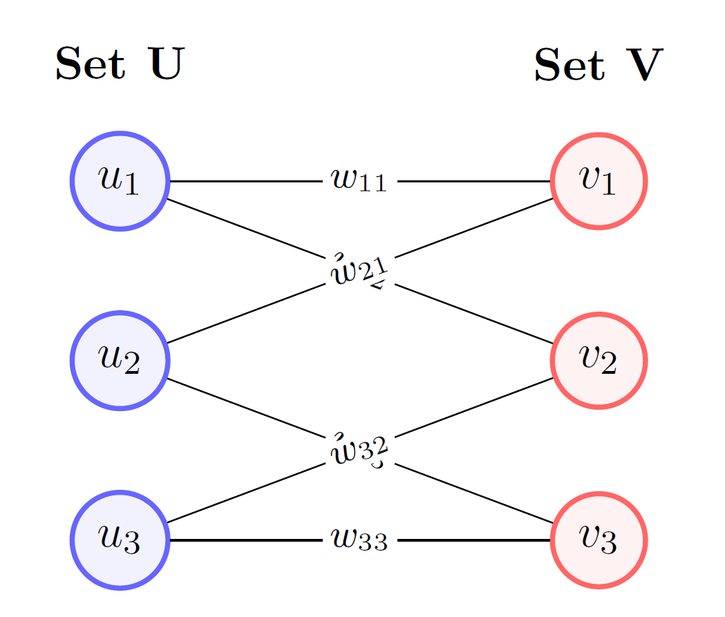
Mathematically, we want to solve the following optimization problem: where is the set of all perfect matchings in . This can be represented using a cost matrix of size , where . The goal is to select one element from each row and each column such that the sum of the selected elements is minimized .
The Hungarian algorithm leverages the concept of a feasible labeling and an equality subgraph . A feasible labeling is a function such that for every edge : The equality subgraph for a given feasible labeling is the subgraph of containing only the edges for which the feasible labeling condition holds with equality: A key theorem, due to Kuhn and Munkres, states that if a perfect matching exists in an equality subgraph , then is a minimum weight perfect matching in the original graph . The Hungarian algorithm iteratively adjusts the feasible labeling and searches for a perfect matching in the corresponding equality subgraph . The algorithm proceeds by initializing a feasible labeling and an empty matching . It then tries to find an augmenting path in the current equality subgraph . If an augmenting path is found, the matching is augmented . If not, the algorithm updates the feasible labeling to create new edges in the equality subgraph, guaranteeing that an augmenting path can be found in a future iteration . This process continues until a perfect matching is found.
The Hungarian Algorithm #
The algorithm can be summarized in the following steps . We start with an initial feasible labeling, for instance, for all and for all .
Algorithm: The Hungarian Matching Algorithm

Here’s a breakdown of the matrix-based method and why it works . Given a cost matrix of size , we want to find a permutation of that minimizes the total cost . This is equivalent to finding a perfect matching of minimum weight in a weighted bipartite graph .
Step 1: Cost Matrix Reduction (Creating Zeros) #
- Action:
- For each row, find the minimum element and subtract it from every element in that row .
- For each column in the resulting matrix, find the minimum element and subtract it from every element in that column .
- Why it’s done: The goal is to create as many zero-entries as possible . A zero in the matrix represents a “free” assignment—an assignment that, relative to the other options in its row and column, is the best possible . If we can find a complete assignment (a set of independent zeros, one in each row and column), we have found an optimal solution .
- Mathematical Justification: This step does not change the set of optimal assignments . Consider subtracting a value from every element in row . Any valid assignment must select exactly one element from row . Therefore, the total cost of any possible perfect matching is reduced by exactly . Since the cost of all possible assignments is reduced by the same amount, the assignment that was optimal before the subtraction remains optimal afterward . The same logic applies to subtracting a value from each column . Formally, if is the new cost matrix after subtracting row-minimums and column-minimums , the cost of any perfect matching in is related to its cost in by: Since and are constants, minimizing is equivalent to minimizing . By performing these reductions, we create a non-negative matrix where the optimal solution has a cost of zero .
Step 2: Find the Maximum Number of Independent Zeros #
- Action: Find the largest possible set of zeros where no two zeros share the same row or column . In the procedural algorithm, this is done by “starring” such zeros .
- Why it’s done: We are testing if the zeros we currently have are sufficient to form a complete, optimal assignment .
- Mathematical Justification: This is equivalent to finding a maximum matching in the bipartite graph where an edge exists only for zero-cost assignments . If we find independent zeros, we have found a perfect matching in this “zero-cost” graph . Because all costs in the reduced matrix are non-negative, this zero-cost assignment must be optimal . If we find fewer than independent zeros, no perfect matching is possible with the current set of zeros, and we must proceed .
Step 3: Cover Zeros with Minimum Lines #
- Action: Draw the minimum number of horizontal and vertical lines required to cover all the zeros in the matrix .
- Why it’s done: This is a crucial diagnostic step . The number of lines tells us the maximum number of independent zeros we can select . If the number of lines is less than , we need to create more zeros to find a complete assignment .
- Mathematical Justification: This step is a direct application of Kőnig’s Theorem . The theorem states that in any bipartite graph, the number of edges in a maximum matching is equal to the minimum number of vertices required to cover all edges . In our matrix context, the “vertices” are the rows and columns, and the “edges” are the positions of the zeros . Therefore, the minimum number of lines needed to cover all zeros is equal to the maximum number of independent zeros . If this number, , is less than , we know a perfect matching is not yet possible .
Step 4: Create New Zeros (Matrix Adjustment) #
- Action:
- Find the smallest element, , that is not covered by any line .
- Subtract from all uncovered elements and add it to all elements at the intersection of two lines .
- Why it’s done: This step intelligently modifies the cost matrix to introduce at least one new zero, creating new opportunities for an assignment . It does this while preserving the existing zeros and ensuring no negative costs are created .
- Mathematical Justification: This is the most complex step and is equivalent to updating the feasible labels in the dual formulation of the assignment problem . Let’s analyze the effect on cell values:
- Uncovered cells: Value decreases by . One of them will become a new zero.
- Singly-covered cells: Value is unchanged. This preserves our existing zeros .
- Doubly-covered cells: Value increases by . This prevents them from becoming negative and maintains feasibility . This procedure guarantees that we make progress towards the solution . By creating a new zero, we either increase the size of the maximum matching or change the line-covering structure, leading to a different in the next iteration .
Repetition #
The algorithm repeats Steps 2, 3, and 4 until the minimum number of lines required to cover all zeros is equal to . At that point, a perfect matching consisting of independent zeros exists and is the optimal solution .
Hungarian Matching for Set‐Prediction (short) #
In many modern models (e.g. DETR, Slot Attention), we have an unordered set of predictions
and an unordered set of ground‐truth targets
To compute a training loss, we need a one‐to‐one correspondence between and . We do this by solving the assignment problem via the Hungarian (Kuhn-Munkres) algorithm.
Problem Formulation #
Define a cost function
e.g. negative log‐likelihood for class label matching plus an distance on attributes. Form the cost matrix
We seek a permutation minimizing the total cost:
Once is found, the supervised loss is
where is the chosen per‐pair loss (e.g. cross‐entropy or regression loss) .
The Hungarian Algorithm #
The Hungarian algorithm solves the above in time . Its main stages are:
- Row reduction: For each row , subtract from all entries in row .
- Column reduction: For each column , subtract from all entries in column .
- Zero covering: Cover all zeros in the matrix using the minimum number of horizontal and vertical lines .
- Adjustment: If fewer than lines are used, let be the smallest uncovered entry; subtract from all uncovered entries and add to entries covered twice. Repeat zero‐covering .
- Assignment: Once zeros can be covered with lines, select zeros so that no two are in the same row or column . These positions give the optimal .
Algorithm 2: Hungarian Algorithm for the Assignment Problem
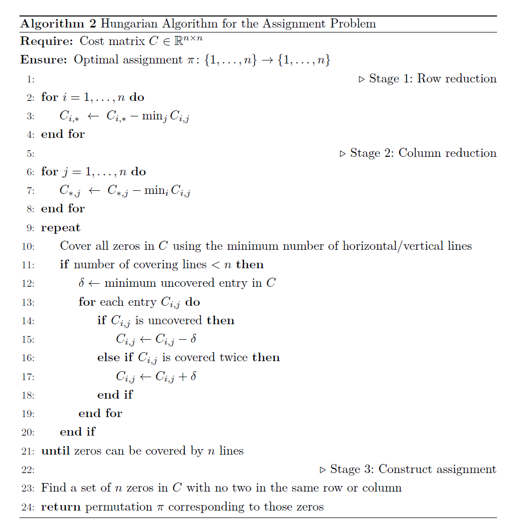
Complexity. Overall, the method runs in time and yields the globally optimal matching in the original cost matrix .
This matching is typically implemented via scipy.optimize.linear_sum_assignment in Python, and is run at each training iteration to align predictions with ground truth before applying the supervised loss .
References #
[1] R. Veerapaneni, J. D. Co-Reyes, M. Chang, M. Janner, C. Finn, J. Wu, J. Tenenbaum, and S. Levine, “Entity Abstraction in Visual Model-Based Reinforcement Learning,” in Proceedings of the Conference on Robot Learning (CoRL), 2020, vol. 100, pp. 1439–1456.
[2] A. Sánchez-González, J. Godwin, T. Pfaff, R. Ying, J. Leskovec, and P. W. Battaglia, “Learning to Simulate Complex Physics with Graph Networks,” in Proceedings of the International Conference on Machine Learning (ICML), 2020, pp. 8459–8468.
[3] M. A. Weis, K. Chitta, Y. Sharma, W. Brendel, M. Bethge, A. Geiger, and A. S. Ecker, “Benchmarking Unsupervised Object Representations for Video Sequences,” Journal of Machine Learning Research, vol. 22, no. 165, pp. 1–27, 2021.
[4] F. Locatello, D. Weissenborn, T. Unterthiner, A. Mahendran, G. Heigold, J. Uszkoreit, A. Dosovitskiy, and T. Kipf, “Object-Centric Learning with Slot Attention,” in Advances in Neural Information Processing Systems (NeurIPS), 2020, vol. 33, pp. 14818–14830.
[5] M. Engelcke, A. R. Kosiorek, O. Parker Jones, and I. Posner, “GENESIS: Generative Scene Inference and Sampling with Object-Centric Latent Representations,” arXiv preprint arXiv:1907.13052, 2020.
[6] M. Engelcke, O. Parker Jones, and I. Posner, “GENESIS-V2: Inferring Unordered Object Representations without Iterative Refinement,” in Advances in Neural Information Processing Systems (NeurIPS), 2021.
[7] C. P. Burgess, L. Matthey, N. Watters, R. Kabra, I. Higgins, M. Botvinick, and A. Lerchner, “MONet: Unsupervised Scene Decomposition and Representation,” arXiv preprint arXiv:1901.11390, 2019.
[8] R. Girdhar and D. Ramanan, “CATER: A Diagnostic Dataset for Compositional Actions and Temporal Reasoning,” arXiv preprint arXiv:1910.04744, 2020.
[9] K. Kim, Y. Park, and M. Jeon, “Emergence of Grid-Like Representations in Recurrent Neural Networks for Spatial Navigation,” Sensors, vol. 23, no. 4, pp. 1–18, 2023.
[10] S. Driess, et al., “PaLM-E: An Embodied Multimodal Language Model,” arXiv preprint arXiv:2303.03378, 2023.
[11] S. Reed, et al., “A Generalist Agent,” arXiv preprint arXiv:2205.06175, 2022.
[12] H. Xu, et al., “VideoCLIP: Contrastive Pretraining for Zero-Shot Video-Text Understanding,” in Proceedings of the Conference on Empirical Methods in Natural Language Processing (EMNLP), 2021, pp. 6780–6791.
[13] A. Anandkumar, H. Pfister, and Y. Li, “Dojo: A Differentiable Physics Engine for Learning and Control,” in Proceedings of the International Conference on Learning Representations (ICLR), 2022.
[14] Z. Mo, et al., “PartNet-Mobility: A Dataset of 3D Articulated Objects,” in Proceedings of the IEEE/CVF Conference on Computer Vision and Pattern Recognition (CVPR), 2021, pp. 11916–11925.
[15] B. Calli, A. Singh, J. Bruce, A. Walsman, K. Konolige, and P. Abbeel, “YCB Object and Model Set: Towards Common Benchmarks for Manipulation Research,” in Proceedings of the International Conference on Advanced Robotics (ICAR), 2015, pp. 510–517.
[16] Y. He, et al., “ARNOLD: A Benchmark for Language-Grounded Task Learning with Continuous States and Actions,” in Proceedings of the Conference on Robot Learning (CoRL), 2022, pp. 2423–2431.
[17] A. Rajeshwaran, Y. Lu, K. Hausman, V. Kumar, G. Gharti R, P. J. Ball, H. Su, and S. Levine, “Robonet: Large-scale Multi-Robot Learning,” arXiv preprint arXiv:2006.10666, 2020.
[18] T. Yu, C. Finn, D. Bahdanau, E. Imani, and S. Levine, “Meta-World: A Benchmark and Evaluation for Multi-Task and Meta Reinforcement Learning,” arXiv preprint arXiv:1910.10897, 2020.
[19] X. Lin, Y. Li, Y. Wang, Z. Xu, S. Levine, and Y. Kuniyoshi, “ManiSkill2: A Benchmark for Generalizable Manipulation Skill Learning,” in Advances in Neural Information Processing Systems (NeurIPS), 2022.
[20] A. Zeng, S. Song, K.-T. Yu, E. H. Lockerman, J. Kozan, A. Irpan, S. Chang, D. Held, and T. H. Fang, “Transporter Networks: Rearranging the Visual World for Robotic Manipulation,” in IEEE International Conference on Robotics and Automation (ICRA), 2020.
[21] A. Zeng, S. Song, K.-T. Yu, E. H. Lockerman, J. Kozan, A. Irpan, S. Chang, D. Held, and T. H. Fang, “SE(3)-Transporter Networks for 6-DoF Robotic Manipulation,” arXiv preprint arXiv:2201.04403, 2022.
[22] Y. Zhang, W. Li, G. Zha, L. Manuelli, D. Fox, and Y. Zhu, “Visual Pretraining with Slot Attention for Robotic Manipulation,” arXiv preprint arXiv:2302.05640, 2023.
[23] X. Qin, P. Xu, K. Dwivedi, D. Gu, and Y. Zhu, “CLEAR: Compositional Learning of Object-centric Agent Representations for Robotics,” arXiv preprint arXiv:2303.05701, 2023.