Message Passing & Aggregation

Message Passing & Aggregation

Author: Christoph Würsch, ICE

A Comparative Analysis of GraphSAGE, HAN, and HGT Graph Neural Networks

Table of Contents

• Core GNN Concepts: Message Passing & Aggregation
• GraphSAGE (Graph Sample and Aggregate)
  • Mathematical Formulation
• HAN (Heterogeneous Graph Attention Network)
  • Mathematical Formulation
  • Step 1: Node-Level Attention
  • Step 2: Semantic-Level Attention
  • Instructive Example: Scientific Collaboration Network
• HGT (Heterogeneous Graph Transformer)
  • Mathematical Formulation
• Conclusion
• References

donwnload as pdf

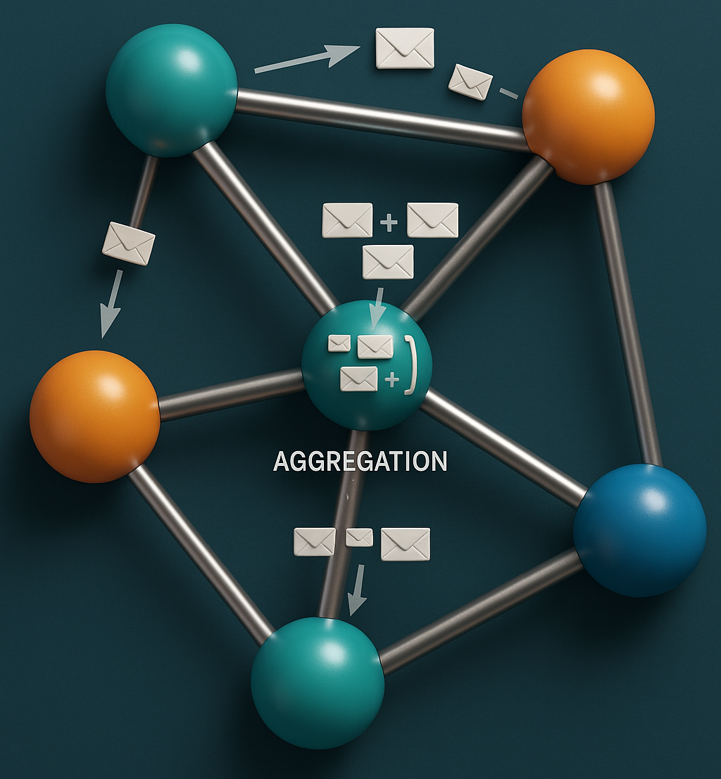
Core GNN Concepts: Message Passing & Aggregation

At their core, most GNNs operate on a neighborhood aggregation or message passing framework. This process allows nodes to iteratively update their feature representations (embeddings) by incorporating information from their local neighborhoods. A single layer of a GNN can be generally described by three key steps:

1. Message Passing: For a target node $v$, each neighboring node $u \in \mathcal{N}(v)$ generates a “message” $m_{u \to v}$. This message is typically a function of the neighbor’s feature vector $h_u$.

2. Aggregation: The target node $v$ aggregates all incoming messages from its neighbors into a single vector, $m_{\mathcal{N}(v)}$. The AGGREGATE function must be permutation-invariant (e.g., sum, mean, max) as the order of neighbors is irrelevant.

   $$m_{\mathcal{N}(v)} = \text{AGGREGATE}(\{m_{u \to v} : u \in \mathcal{N}(v)\})$$

3. Update: The node $v$ updates its own embedding $h_v$ by combining its previous embedding $h_v^{k-1}$ with the aggregated message $m_{\mathcal{N}(v)}$.

   $$h_v^k = \text{UPDATE}(h_v^{k-1}, m_{\mathcal{N}(v)})$$

   Here, $k$ denotes the $k$-th layer of the GNN. The models we discuss below are specific instantiations of this general framework.

GraphSAGE (Graph Sample and Aggregate)

GraphSAGE [1] was designed to be a general, inductive framework that can generate embeddings for previously unseen nodes. Its key innovation is not training on the full graph but on sampled local neighborhoods. The primary innovation of GraphSAGE is its inductive capability, which allows it to generalize to previously unseen nodes. This makes it exceptionally well-suited for dynamic, large-scale graphs where the entire graph structure is not available during training.

One of the most prominent applications is in the domain of social networks and content recommendation. In the original paper, GraphSAGE was used for node classification on the Reddit dataset to classify post topics [1]. A landmark industrial application is PinSAGE, a GNN-based recommender system developed by Pinterest. PinSAGE uses GraphSAGE’s principles to recommend “pins” (images) to users by learning embeddings for billions of items in a dynamic web-scale graph. It effectively handles the challenge of generating recommendations for new, unseen content on a daily basis [2]. Its success has made it a blueprint for modern GNN-based recommender systems.

Instead of using the entire neighborhood for aggregation, GraphSAGE uniformly samples a fixed-size set of neighbors at each layer. This ensures that the computational footprint for each node is fixed, making the model scalable to massive graphs. GraphSAGE is primarily designed for homogeneous graphs, where all nodes and edges are of the same type.

Mathematical Formulation

For a target node $v$ at layer $k$, the process is as follows:

1. Sample Neighborhood: Sample a fixed-size neighborhood $\mathcal{N}_S(v)$ from the full set of neighbors $\mathcal{N}(v)$.
2. Aggregate: Aggregate the feature vectors from the sampled neighbors. The Mean aggregator is a common choice: $$h_{\mathcal{N}_S(v)}^k = \frac{1}{|\mathcal{N}_S(v)|} \sum_{u \in \mathcal{N}_S(v)} h_u^{k-1}$$
3. Update: Concatenate the node’s own representation from the previous layer, $h_v^{k-1}$, with the aggregated neighbor vector. This combined vector is then passed through a fully connected layer with a non-linear activation function $\sigma$. $$h_v^k = \sigma \left( \mathbf{W}^k \cdot \text{CONCAT}(h_v^{k-1}, h_{\mathcal{N}_S(v)}^k) \right)$$ where $\mathbf{W}^k$ is a trainable weight matrix for layer $k$.

HAN (Heterogeneous Graph Attention Network)

HAN [3] is specifically designed to work with heterogeneous graphs, which contain multiple types of nodes and edges. It acknowledges that different types of nodes and relationships contribute differently to a task. HAN’s strength lies in its ability to leverage predefined semantic relationships (meta-paths) to generate task-aware node representations in heterogeneous graphs. This is particularly useful in domains where expert knowledge can guide the model’s focus.

The canonical application for HAN is in academic network analysis. As demonstrated in the original paper, HAN can effectively classify research papers or authors in bibliographic networks like DBLP and ACM by utilizing meta-paths such as Author-Paper-Author (co-authorship) and Author-Paper-Subject-Paper-Author (shared research topics) [3]. Another critical application area is fraud and anomaly detection. In financial or e-commerce networks, relationships between users, devices, IP addresses, and transactions are heterogeneous. By defining meta-paths that capture known fraudulent patterns (e.g., User-Device-User), HAN can learn powerful embeddings to identify malicious actors. While many industrial systems are proprietary, research from companies like Alibaba has shown the power of heterogeneous GNNs for this purpose [4].

HAN uses a hierarchical attention mechanism. First, node-level attention learns the importance of different neighbors within a specific relationship type (meta-path). Second, semantic-level attention learns the importance of the different meta-paths themselves. A meta-path is a sequence of relations connecting two node types (e.g., Author $\rightarrow$ Paper $\rightarrow$ Author).

Mathematical Formulation

Let $\Phi_i$ be a meta-path.

1. Node-Level Attention: For a node $v$ and its neighbors $\mathcal{N}_v^{\Phi_i}$ connected via meta-path $\Phi_i$, HAN learns attention weights $\alpha_{vu}^{\Phi_i}$ for each neighbor $u \in \mathcal{N}_v^{\Phi_i}$. The embedding for node $v$ specific to this meta-path is an aggregation of its neighbors’ features, weighted by attention: $$z_v^{\Phi_i} = \sum_{u \in \mathcal{N}_v^{\Phi_i}} \alpha_{vu}^{\Phi_i} \cdot h_u$$
2. Semantic-Level Attention: After obtaining semantic-specific embeddings $\{z_v^{\Phi_1}, \dots, z_v^{\Phi_P}\}$, HAN learns weights $(\beta_{\Phi_1}, \dots, \beta_{\Phi_P})$ for each meta-path. The final embedding $Z_v$ is a weighted sum: $$Z_v = \sum_{i=1}^{P} \beta_{\Phi_i} \cdot z_v^{\Phi_i}$$

A meta-path is a predefined sequence of node types and edge types that describes a composite relationship (a “semantic path”) between two nodes. For example, in a scientific collaboration network with Authors (A), Papers (P), and Subjects (S), a meta-path Author-Paper-Author (APA) represents the co-author relationship. Another meta-path, Author-Paper-Subject-Paper-Author (APSPA), could represent the relationship between two authors who have written papers on the same subject. HAN leverages these user-defined paths to group neighbors by semantics.

Step 1: Node-Level Attention

The first level of attention aims to answer the question: Within a single semantic path, which neighbors are most important for a given node?

For a specific meta-path $\Phi_i$, a central node $v$ has a set of neighbors $\mathcal{N}_v^{\Phi_i}$. The node-level attention mechanism learns to assign different importance weights to these neighbors.

1. Feature Transformation: Since different node types may have different feature spaces, their initial feature vectors ($h_v$) are first projected into a common space using a type-specific transformation matrix $\mathbf{M}_{\tau_v}$, where $\tau_v$ is the type of node $v$. For simplicity in this explanation, we assume features are already in a common space.

2. Attention Coefficient Calculation: For a pair of nodes $(v, u)$ connected via meta-path $\Phi_i$, the attention coefficient $e_{vu}^{\Phi_i}$ is calculated. This measures the importance of node $u$ to node $v$. It is parameterized by a learnable attention vector $\mathbf{a}_{\Phi_i}$ specific to the meta-path:

   $$e_{vu}^{\Phi_i} = \text{LeakyReLU}\left( \mathbf{a}_{\Phi_i}^T \cdot [\mathbf{W}h_v || \mathbf{W}h_u] \right)$$

   where $\mathbf{W}$ is a shared linear transformation matrix applied to the features of each node, and $||$ denotes concatenation.

3. Normalization: The attention coefficients are then normalized across all neighbors of node $v$ using the softmax function to obtain the final attention weights $\alpha_{vu}^{\Phi_i}$. These weights represent a probability distribution of importance over the neighbors.

   $$\alpha_{vu}^{\Phi_i} = \text{softmax}_u(e_{vu}^{\Phi_i}) = \frac{\exp(e_{vu}^{\Phi_i})}{\sum_{k \in \mathcal{N}_v^{\Phi_i}} \exp(e_{vk}^{\Phi_i})}$$

4. Aggregation: Finally, the semantic-specific embedding for node $v$, $z_v^{\Phi_i}$, is computed as a weighted sum of its neighbors’ transformed features.

   $$z_v^{\Phi_i} = \sigma\left( \sum_{u \in \mathcal{N}_v^{\Phi_i}} \alpha_{vu}^{\Phi_i} \cdot \mathbf{W}h_u \right)$$

   where $\sigma$ is a non-linear activation function (e.g., ELU).

This process is repeated for every defined meta-path, resulting in a set of semantic-specific embeddings for each node $\{z_v^{\Phi_1}, z_v^{\Phi_2}, \dots, z_v^{\Phi_P}\}$.

Step 2: Semantic-Level Attention

After obtaining different embeddings for each semantic path, the second level of attention answers the question: For a given node, which semantic path is the most important?

1. Importance Weight Calculation: HAN learns the importance of each meta-path $\Phi_i$ for a node $v$. This is achieved by first transforming each semantic-specific embedding $z_v^{\Phi_i}$ (e.g., through a linear layer and tanh activation) and then measuring its similarity to a shared, learnable semantic-level attention vector $\mathbf{q}$.

   $$w_{\Phi_i} = \frac{1}{|\mathcal{V}|} \sum_{v \in \mathcal{V}} \mathbf{q}^T \cdot \tanh(\mathbf{W}_{sem} z_v^{\Phi_i} + \mathbf{b}_{sem})$$

   where $\mathbf{W}_{sem}$ and $\mathbf{b}_{sem}$ are learnable parameters, and the weights are averaged over all nodes $\mathcal{V}$ in the graph.

2. Normalization: These importance weights are also normalized using a softmax function to obtain the final semantic weights $\beta_{\Phi_i}$.

   $$\beta_{\Phi_i} = \frac{\exp(w_{\Phi_i})}{\sum_{j=1}^{P} \exp(w_{\Phi_j})}$$

3. Final Aggregation: The final node embedding $Z_v$ is a weighted average of all its semantic-specific embeddings, using the learned semantic weights $\beta$.

   $$Z_v = \sum_{i=1}^{P} \beta_{\Phi_i} \cdot z_v^{\Phi_i}$$

This final embedding $Z_v$ is a rich representation that has selectively aggregated information from the most relevant neighbors and the most relevant relationship types.

Instructive Example: Scientific Collaboration Network

Let’s consider a graph with Authors, Papers, and research Subjects. Our goal is to generate an embedding for a target author, Dr. Eva Meyer. We define two meta-paths:

• $\Phi_1 = \texttt{Author-Paper-Author}$ (APA): Represents the co-author relationship.
• $\Phi_2 = \texttt{Author-Paper-Subject-Paper-Author}$ (APSPA): Represents authors working on similar subjects.

Node-Level Attention in Action:

• For meta-path APA, Dr. Meyer’s neighbors are her co-authors: Prof. Schmidt and Dr. Chen. The node-level attention might learn that for predicting future research topics, Prof. Schmidt’s work is more influential. Thus, it assigns a higher weight: $\alpha_{\text{Meyer}, \text{Schmidt}}^{\text{APA}} = 0.7$, $\alpha_{\text{Meyer}, \text{Chen}}^{\text{APA}} = 0.3$. The embedding $z_{\text{Meyer}}^{\text{APA}}$ will therefore be heavily influenced by Prof. Schmidt’s features.
• For meta-path APSPA, Dr. Meyer’s neighbors are authors who publish on the same subjects, like Dr. Lee and Prof. Ivanova. Here, the attention might find both to be equally important, resulting in weights like $\alpha_{\text{Meyer}, \text{Lee}}^{\text{APSPA}} = 0.5$ and $\alpha_{\text{Meyer}, \text{Ivanova}}^{\text{APSPA}} = 0.5$.

Semantic-Level Attention in Action: Dr. Meyer now has two embeddings: $z_{\text{Meyer}}^{\text{APA}}$ (representing her collaborative circle) and $z_{\text{Meyer}}^{\text{APSPA}}$ (representing her subject-matter community).

• If the downstream task is to recommend new collaborators, the direct co-author relationship is likely more important. The semantic-level attention might learn weights: $\beta_{\text{APA}} = 0.8$, $\beta_{\text{APSPA}} = 0.2$.
• If the task is to classify her research field, the community of authors working on similar topics might be more telling. The weights could be: $\beta_{\text{APA}} = 0.3$, $\beta_{\text{APSPA}} = 0.7$.

The final embedding $Z_{\text{Meyer}}$ is then computed as $Z_{\text{Meyer}} = \beta_{\text{APA}} \cdot z_{\text{Meyer}}^{\text{APA}} + \beta_{\text{APSPA}} \cdot z_{\text{Meyer}}^{\text{APSPA}}$, providing a task-aware representation of Dr. Meyer.

HGT (Heterogeneous Graph Transformer)

HGT [5] is a more recent and dynamic approach for heterogeneous graphs. It adapts the powerful Transformer architecture to graphs, avoiding the need for pre-defined meta-paths. HGT excels where relationships are numerous and dynamic, and defining all meaningful meta-paths is impractical. By parameterizing its attention mechanism based on node and edge types, it can dynamically learn the importance of different relationships without prior specification.

Like HAN, HGT has shown state-of-the-art results in academic network analysis, particularly for node classification in large, evolving bibliographic datasets [5]. Its key advantage is not needing to pre-specify meta-paths, allowing it to discover novel, important relationships on its own. A rapidly growing application area for HGT is in knowledge graph completion and recommendation. In large-scale knowledge graphs (e.g., Freebase, Wikidata) or e-commerce product graphs, the number of node and edge types can be in the hundreds or thousands. HGT’s dynamic, type-aware attention mechanism is highly effective at modeling these complex interactions to predict missing links or recommend products to users based on a wide variety of relationships (e.g., user-viewed-product, product-in-category, product-by-brand).

HGT models heterogeneity by parameterizing the weight matrices in its attention mechanism based on node and edge types. For any two nodes and the edge between them, HGT computes attention in a way that is specific to their types, allowing for a more flexible and direct modeling of interactions.

Mathematical Formulation

The core of HGT is its Heterogeneous Mutual Attention mechanism. To calculate the message from a source node $s$ to a target node $t$ at layer $k$:

1. Type-Specific Projections: Project features into Query, Key, and Value vectors using type-specific matrices. Let $\tau(n)$ be the type of node $n$ and $\phi(s, t)$ be the type of edge $(s,t)$. $$\begin{align*} \text{Query}(t) &= \mathbf{W}_Q^{\tau(t)} h_t^{k-1} \\ \text{Key}(s) &= \mathbf{W}_K^{\tau(s)} h_s^{k-1} \end{align*}$$
2. Attention Calculation: Use a scaled dot-product attention that also incorporates an edge-type-specific matrix $\mathbf{W}_{\phi(s,t)}$. $$\alpha(s, t) = \text{softmax}_{s \in \mathcal{N}(t)} \left( \frac{(\text{Query}(t))^T \mathbf{W}_{\phi(s,t)} \text{Key}(s)}{\sqrt{d}} \right)$$
3. Message Calculation & Aggregation: Aggregate messages from all neighbors. $$\tilde{h}_t^k = \sum_{s \in \mathcal{N}(t)} \alpha(s, t) \cdot (\mathbf{W}_V^{\tau(s)} h_s^{k-1})$$
4. Update: Use a residual connection, similar to a standard Transformer block. $$h_t^k = \text{LayerNorm}(h_t^{k-1} + \text{Linear}(\tilde{h}_t^k))$$

High-level comparison of GraphSAGE, HAN, and HGT

GraphSAGE, HAN, and HGT represent a clear progression in GNN design. GraphSAGE provides a powerful and scalable baseline for homogeneous graphs. HAN introduces a sophisticated way to handle heterogeneity by incorporating domain knowledge through meta-paths. HGT builds upon this by removing the dependency on pre-defined meta-paths, using a more flexible and powerful Transformer-based attention mechanism that dynamically learns the importance of different types of relationships directly from the graph structure. The choice between them depends on the nature of the graph data: for simple, homogeneous graphs, GraphSAGE is a strong choice, while for complex, heterogeneous graphs, HGT often provides superior performance due to its dynamic and expressive architecture.

References

1. Hamilton, W. L., Ying, R., & Leskovec, J. (2017). Inductive representation learning on large graphs. In Advances in neural information processing systems (NIPS).

2. Ying, R., He, R., Chen, K., Eksombatchai, P., Hamilton, W. L., & Leskovec, J. (2018). Graph convolutional neural networks for web-scale recommender systems. In Proceedings of the 24th ACM SIGKDD international conference on knowledge discovery & data mining.

3. Wang, X., Ji, H., Shi, C., Wang, B., Cui, P., Yu, P. S., & Ye, Y. (2019). Heterogeneous graph attention network. In The World Wide Web Conference (WWW).

4. Liu, Z., Chen, C., Yang, X., Zhou, J., Li, X., & Song, L. (2020). Heterogeneous graph neural networks for malicious account detection. In Proceedings of the 29th ACM international conference on information & knowledge management (CIKM).

5. Hu, Z., Dong, Y., Wang, K., & Sun, Y. (2020). Heterogeneous graph transformer. In Proceedings of The Web Conference (WWW).