The Spectral Mixture (SM) Kernel

The Spectral Mixture (SM) Kernel for Gaussian Processes

Author: Christoph Würsch, ICE, Eastern Switzerland University of Applied Sciences, OST

Table of Contents

• The Gaussian Process as a Distribution over Functions
  • The Kernel as a High-Dimensional Covariance Matrix
  • The RBF Kernel: The ”Workhorse” of GPs
  • The Limitations of Standard Kernels
• The Spectral Mixture (SM) Kernel
  • The Spectral Perspective: Bochner’s Theorem
  • The Spectral Mixture (SM) Kernel
  • Pattern Discovery and Extrapolation
    • Example: The $CO_2$ Dataset
  • Implementation and Practical Issues
    • A Critical Caveat: Initialization
• Take Aways

The Gaussian Process as a Distribution over Functions

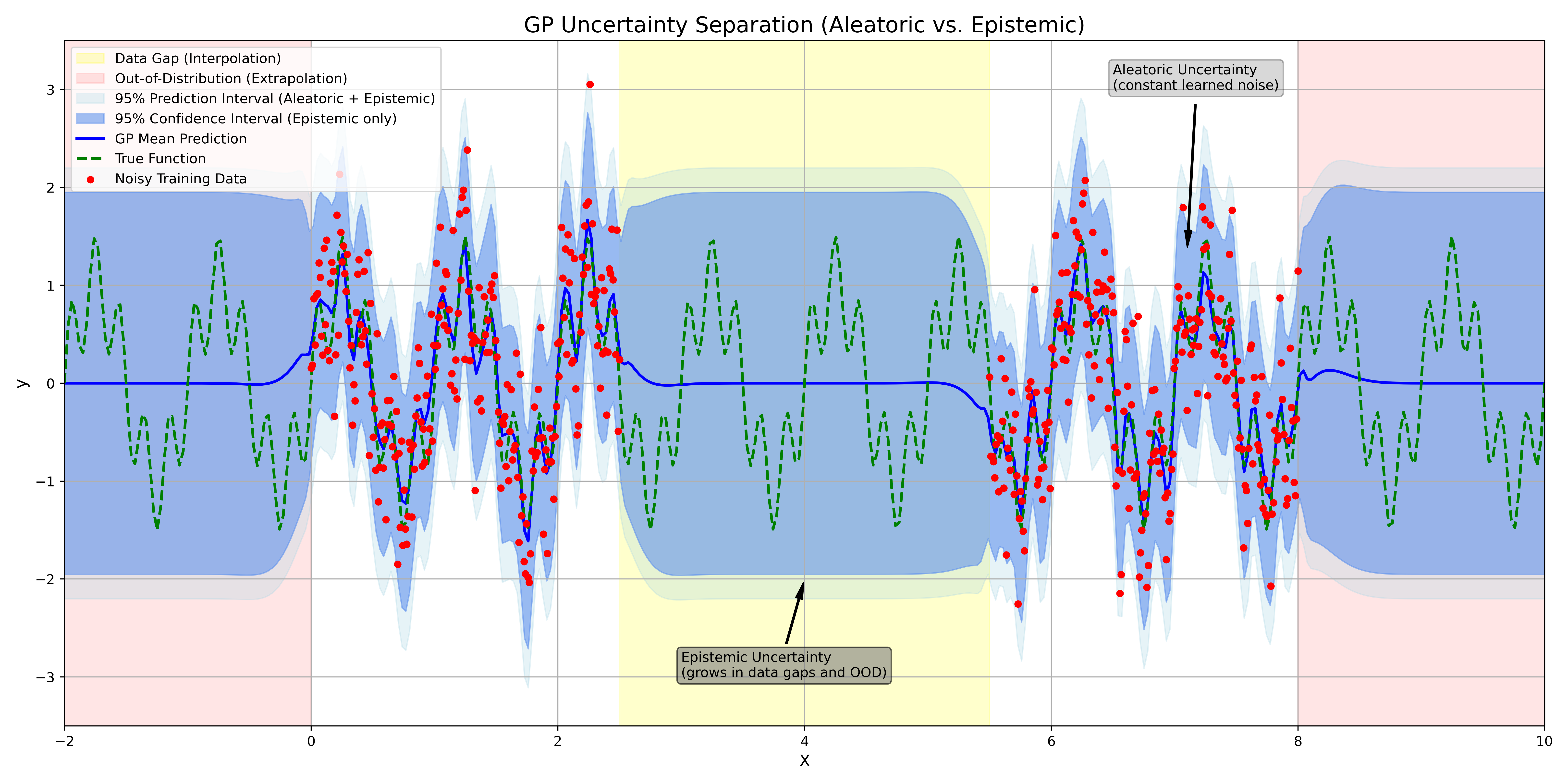
In the realm of machine learning, most models are parametric; they are defined by a set of parameters $\boldsymbol{\theta}$ (e.g., the weights of a neural network), and our goal is to find the optimal $\boldsymbol{\theta}$ based on the data. Gaussian Processes (GPs) [1] offer a fundamentally different, non-parametric perspective. Instead of learning parameters for a specific function, a Gaussian Process places a probability distribution directly over the space of all possible functions. This ”distribution over functions” provides a powerful and principled framework for Uncertainty Quantification (UQ). A GP does not just yield a single point prediction $y^*$; it provides an entire Gaussian distribution $\mathcal{N}(\mu^*, \sigma^{2*})$ for any new input $\mathbf{x}^*$, where $\mu^*$ is the most likely prediction and $\sigma^{2*}$ explicitly quantifies the model’s uncertainty about that prediction. Formally, a Gaussian Process is defined as follows:

Definition A Gaussian Process (GP) is a collection of random variables, any finite number of which have a joint Gaussian distribution.

A GP is fully specified by a mean function $m(\mathbf{x})$ and a covariance function $k(\mathbf{x}, \mathbf{x}')$:

The mean function $m(\mathbf{x}) = \mathbb{E}[f(\mathbf{x})]$ represents the expected value of the function at input $\mathbf{x}$. For simplicity, this is often assumed to be zero, $m(\mathbf{x}) = 0$, after centering the data. The true ”heart” of the GP is the covariance function, or kernel, $k(\mathbf{x}, \mathbf{x}') = \text{Cov}(f(\mathbf{x}), f(\mathbf{x}'))$. The kernel’s role is to encode our prior assumptions about the function’s properties, such as its smoothness, stationarity, or periodicity. It defines the ”similarity” between the function’s output at two different points, $\mathbf{x}$ and $\mathbf{x}'$. If two points are ”similar” according to the kernel, their function values are expected to be highly correlated.

The Kernel as a High-Dimensional Covariance Matrix

The definition of a GP elegantly connects the infinite-dimensional concept of a ”function” to the finite-dimensional mathematics we use for computation. Given a finite dataset of $N$ input points, $\mathbf{X} = \{\mathbf{x}_1, \dots, \mathbf{x}_N\}$, the joint distribution of the corresponding function values $\mathbf{f} = [f(\mathbf{x}_1), \dots, f(\mathbf{x}_N)]^T$ is, by definition, a high-dimensional Multivariate Gaussian. The covariance matrix $\mathbf{K}$ of this Multivariate Gaussian is constructed by evaluating the kernel function at every pair of points in our dataset:

Thus, our prior belief about the function $f$ at the points $\mathbf{X}$ is expressed as:

The choice of kernel $k$ entirely determines the $N \times N$ covariance matrix $\mathbf{K}$, which in turn defines the properties of all functions sampled from this prior.

The RBF Kernel: The ”Workhorse” of GPs

While countless kernels exist, the most common and arguably most important is the Radial Basis Function (RBF) kernel, also known as the Squared Exponential or Gaussian kernel. Its enduring popularity stems from its simplicity and its strong, yet often reasonable, prior assumption: smoothness. The RBF kernel is defined as:

This kernel is defined by two hyperparameters:

• Signal Variance ($\sigma_f^2$): This is an amplitude parameter. It controls the total variance of the function, scaling the covariance values up or down. It represents the maximum expected variation from the mean.
• Lengthscale ($l$): This is the most critical parameter. It defines the ”characteristic distance” over which the function’s values are correlated.

The RBF kernel is stationary (it depends only on the distance $||\mathbf{x}_i - \mathbf{x}_j||$, not on the absolute locations) and infinitely smooth. A small lengthscale $l$ means the correlation drops off quickly, allowing the function to vary rapidly. A large $l$ means that even distant points are correlated, resulting in a very smooth, slowly varying function. When we use an RBF kernel, we are placing a prior on functions that we believe to be smooth. The core idea of GP regression, which we will explore in the following sections, is to take this high-dimensional Gaussian prior $\mathcal{N}(\mathbf{0}, \mathbf{K})$built from our RBF kerneland condition it on our finite set of noisy observations $\mathcal{D} = \{(\mathbf{X}, \mathbf{y})\}$. This conditioning step updates our prior belief, yielding a posterior Gaussian Process that provides both the mean prediction and, crucially for UQ, the predictive uncertainty at any unobserved location.

The Limitations of Standard Kernels

In the application of Gaussian Processes (GPs), we have seen that the choice of kernel $k(\mathbf{x}, \mathbf{x}')$ is paramount. It encodes all our prior assumptions about the function $f(\mathbf{x})$ we are modeling. A popular and widely-used kernel is the Radial Basis Function (RBF) kernel, also known as the Squared Exponential:

where $\tau = ||\mathbf{x} - \mathbf{x}'||$ is the distance between inputs, $\sigma_f^2$ is the signal variance, and $l$ is the characteristic lengthscale. The RBF kernel is a ”universal” kernel in the sense that it can approximate any continuous function given enough data. However, its implicit assumptions are very strong. The RBF kernel is infinitely smooth and stationary. Its primary assumption is that ”nearness” in the input space implies ”nearness” in the output space. This makes it an excellent choice for interpolation and smoothing.

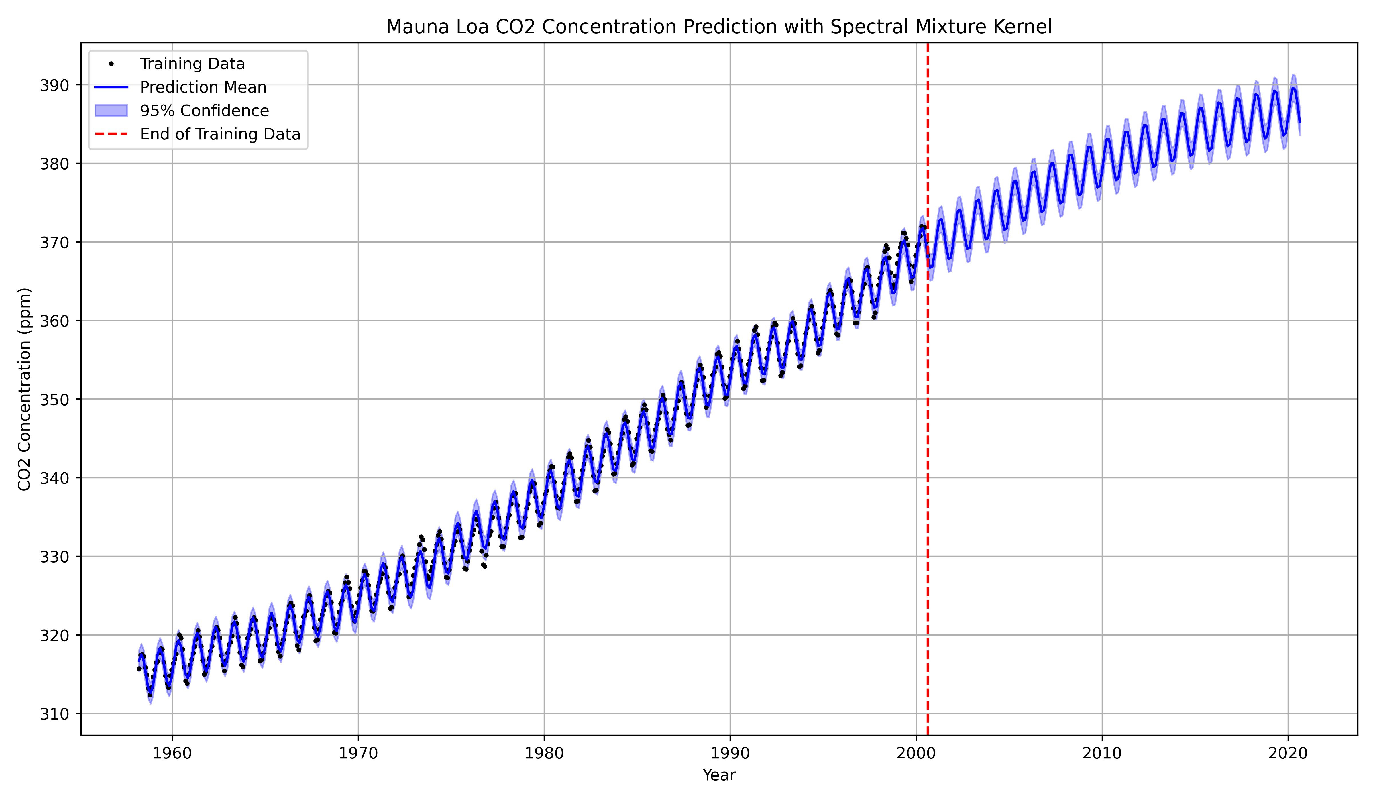
Its weakness, however, is revealed in extrapolation and pattern discovery. Consider the famous Mauna Loa $CO_2$ dataset, which exhibits a clear long-term upward trend combined with a strong annual periodicity.

• An RBF kernel can model the long-term trend, but it will fail to capture the periodicity. When asked to extrapolate, its prediction will revert to the mean.
• A Periodic kernel can capture the seasonality, but it must be multiplied by an RBF kernel to allow for local variations, and crucially, the user must specify the period (e.g., 1 year) in advance. This motivates the need for a kernel that does not just apply a predefined structure (like ”smooth” or ”periodic with period $P$”) but can discover complex, quasi-periodic, and multi-scale patterns directly from the data.

The Spectral Mixture (SM) Kernel [2]

The Spectral Perspective: Bochner’s Theorem

The key to developing a more expressive kernel lies in the frequency domain. A fundamental result in mathematics, Bochner’s Theorem, provides the bridge.

Theorem (Bochner, 1959) A complex-valued function $k(\tau)$ on $\mathbb{R}^D$ is the covariance function of a stationary Gaussian Process if and only if it is the Fourier transform of a non-negative, finite measure $S(\boldsymbol{\omega})$.

For a stationary kernel $k(\boldsymbol{\tau})$ where $\boldsymbol{\tau} = \mathbf{x} - \mathbf{x}'$, this relationship is:

$S(\boldsymbol{\omega})$ is known as the spectral density (or power spectrum) of the kernel. It describes the ”power” or ”strength” of the function at different frequencies $\boldsymbol{\omega}$. Let’s re-examine our standard kernels through this lens:

• RBF Kernel: The spectral density of $k_{\text{RBF}}(\tau)$ is also a Gaussian, centered at zero frequency: $$S_{\text{RBF}}(\omega) \propto \exp\left( -\frac{l^2 \omega^2}{2} \right)$$ This mathematically confirms our intuition: the RBF kernel is a strong low-pass filter. It assumes all the function’s power is concentrated at low frequencies (i.e., the function is smooth).
• Periodic Kernel: The spectral density of a purely periodic kernel is a series of delta functions $\delta(\omega)$ at the fundamental frequency and its harmonics. This is an extremely rigid structure.

The problem is clear: standard kernels have fixed, simple spectral densities. If the true function’s spectrum is complex (e.g., a mix of several periodicities), these kernels will fail to capture it.

The Spectral Mixture (SM) Kernel

The groundbreaking idea of the Spectral Mixture (SM) kernel, introduced by Wilson and Adams (2013) [2], is this: Instead of assuming a fixed spectral density, let’s learn it from the data.

How can we model an arbitrary, non-negative spectral density $S(\omega)$? We can use a Gaussian Mixture Model (GMM), which is a universal approximator for densities. The SM kernel proposes to model the spectral density $S(\omega)$ as a sum of $Q$ Gaussian components. To ensure the resulting kernel $k(\tau)$ is real-valued, the spectrum must be symmetric, $S(\omega) = S(-\omega)$. We thus define the spectral density as a mixture of $Q$ pairs of symmetric Gaussians:

where each component $q$ has a weight $w_q$, a mean frequency $\mu_q$, and a spectral variance $v_q$. Now, we apply Bochner’s theorem and compute the inverse Fourier transform of $S_{\text{SM}}(\omega)$ to find the kernel $k_{\text{SM}}(\tau)$. We use the standard Fourier transform pair:

By applying this to our symmetric GMM and using Euler’s formula ($\cos(x) = \frac{e^{ix} + e^{-ix}}{2}$), the sum of the $q$-th pair of complex exponentials simplifies beautifully into a cosine function. This yields the Spectral Mixture (SM) Kernel for 1D inputs ($\tau = x - x'$):

Spectral Mixture (SM) Kernel (1D)

$$k_{\text{SM}}(\tau) = \sum_{q=1}^Q w_q \cdot \underbrace{\exp(-2\pi^2 v_q \tau^2)}_{\text{RBF-like Component}} \cdot \underbrace{\cos(2\pi \mu_q \tau)}_{\text{Periodic Component}}$$

This kernel is a linear combination of $Q$ components, where each component is a product of an RBF-like kernel and a periodic cosine kernel. The power of the SM kernel comes from the interpretability of its hyperparameters. For each of the $Q$ components, we learn:

• Weight ($w_q$): The component’s overall contribution (amplitude) to the final covariance.
• Mean Frequency ($\mu_q$): The center of the component in the frequency domain. This directly controls the periodicity. The period $P_q$ is $P_q = 1 / \mu_q$.
• Spectral Variance ($v_q$): The variance of the component in the frequency domain. This controls the lengthscale $l_q$ in the time domain ($l_q \propto 1/\sqrt{v_q}$).

This structure allows the kernel to model diverse patterns:

• A smooth trend: A component with $\mu_q \approx 0$ (zero frequency) and large $v_q$ (short lengthscale) behaves like a standard RBF kernel.
• A strong, stable periodicity: A component with $\mu_q > 0$ and very small $v_q$ (long lengthscale) behaves like $\cos(2\pi \mu_q \tau)$.
• A quasi-periodic function: A component with $\mu_q > 0$ and $v_q > 0$ models a wave that slowly ”decays” or changes shape over time.

The kernel can be extended to $D$-dimensional inputs $\mathbf{x} \in \mathbb{R}^D$. We define $\boldsymbol{\tau} = \mathbf{x} - \mathbf{x}'$. Each component $q$ now requires a weight $w_q$, a mean frequency vector $\boldsymbol{\mu}_q \in \mathbb{R}^D$, and a spectral variance vector $\mathbf{v}_q \in \mathbb{R}^D$ (assuming a diagonal covariance $\mathbf{V}_q = \text{diag}(\mathbf{v}_q)$). The multivariate kernel is given by:

Spectral Mixture (SM) Kernel (D-Dimensions)

$$k_{\text{SM}}(\boldsymbol{\tau}) = \sum_{q=1}^Q w_q \exp(-2\pi^2 \boldsymbol{\tau}^T \mathbf{V}_q \boldsymbol{\tau}) \cdot \cos(2\pi \boldsymbol{\mu}_q^T \boldsymbol{\tau})$$

This is a sum of $Q$ components, where each component $k_q$ is a product over the $D$ dimensions:

This structure allows the model to learn different frequencies (e.g., ”daily” in dimension 1, ”weekly” in dimension 2) and different lengthscales for each component in each input dimension.

Pattern Discovery and Extrapolation

The most significant feature of the SM kernel is that the parameters $\{w_q, \boldsymbol{\mu}_q, \mathbf{v}_q\}_{q=1}^Q$ are all hyperparameters of the kernel. Just as we optimize the lengthscale $l$ of an RBF kernel by maximizing the marginal log-likelihood (ML-II), we optimize all $Q \times (2D + 1)$ parameters of the SM kernel. This optimization process is the pattern discovery. The GP automatically fits the GMM to the data’s ”hidden” spectral density.

Example: The $CO_2$ Dataset

If we apply an SM kernel (e.g., with $Q=2$) to the Mauna Loa $CO_2$ data, the optimization will likely find:

• Component 1 (Trend): $w_1 \approx \text{high}$, $\boldsymbol{\mu}_1 \approx \mathbf{0}$, $v_1 \approx \text{small}$ (long lengthscale) This component captures the long-term, non-periodic, smooth upward trend.
• Component 2 (Seasonality): $w_2 \approx \text{medium}$, $\mu_2 \approx 1/\text{year}$, $v_2 \approx \text{very small}$ (very long lengthscale). This component explicitly discovers and isolates the 1-year annual cycle.

Because the model has explicitly learned the periodic component $\cos(2\pi \mu_2 \tau)$, its predictions will extrapolate this pattern into the future, rather than reverting to the mean. This provides state-of-the-art extrapolation for any time-series data that exhibits quasi-periodic behavior (e.g., climate, finance, robotics).

Implementation and Practical Issues

The SM kernel is available in modern probabilistic programming libraries such as GPyTorch.

import torch
import gpytorch

class SpectralMixtureGP(gpytorch.models.ExactGP):
    def __init__(self, train_x, train_y, likelihood, num_mixtures):
    super(SpectralMixtureGP, self).__init__(train_x, train_y, likelihood)

        self.mean_module = gpytorch.means.ConstantMean()

        # Define the Spectral Mixture Kernel
        # num_mixtures is Q
        # ard_num_dims is D (here, 1D input)
        self.covar_module = gpytorch.kernels.SpectralMixtureKernel(
        num_mixtures=num_mixtures,
        ard_num_dims=1
        )

    def forward(self, x):
        mean_x = self.mean_module(x)
        covar_x = self.covar_module(x)
        return gpytorch.distributions.MultivariateNormal(mean_x, covar_x)

#  Example Usage 
# Assume train_x, train_y are 1D tensors
likelihood = gpytorch.likelihoods.GaussianLikelihood()
Q = 4 # We choose to search for 4 components
model = SpectralMixtureGP(train_x, train_y, likelihood, num_mixtures=Q)

# !!
CRITICAL STEP: Initialization !!
# The SM loss landscape is highly multi-modal.
# Random initialization will fail.
We must initialize
# from the data's frequency spectrum (periodogram).
model.covar_module.initialize_from_data(train_x, train_y)

# Now, we train the model as usual
# ... (training loop) ...

A Critical Caveat: InitializationThe SM kernel’s greatest strength (its flexibility) is also its greatest weakness. With $Q \times (2D + 1)$ hyperparameters, the optimization landscape for the marginal log-likelihood is highly multi-modal. A naive or random initialization of the parameters $\{w_q, \boldsymbol{\mu}_q, \mathbf{v}_q\}$ will almost certainly get stuck in a poor local optimum. This kernel is not ”plug-and-play” like an RBF kernel.To use it successfully, one must initialize the parameters intelligently. Libraries like GPyTorch and GPy provide helper functions (e.g., initialize_from_data) that perform the following steps:

1. Compute the empirical spectral density of the data using a periodogram (e.g., via a Fast Fourier Transform, FFT).
2. Fit a GMM to this empirical spectrum.
3. Use the parameters of the fitted GMM (the weights, means, and variances) as the starting values for the kernel’s hyperparameters.

This provides the optimizer with a ”good guess” that is already close to a reasonable solution, allowing it to fine-tune the parameters to the true maximum of the marginal log-likelihood.

Take Aways

The Spectral Mixture kernel is a powerful, expressive tool for Gaussian Process modeling, effectively moving the problem from kernel selection to kernel learning.

When faced with data that exhibits complex, unknown, or quasi-periodic patterns, the SM kernel is one of the most powerful tools in the modern GP toolbox, provided it is used with a proper initialization strategy.

References

[1] Carl Edward Rasmussen and Chris Williams: Gaussian Processes for Machine Learning, the MIT Press, 2006, online

[2] A. G. Wilson and R. P. Adams. ”Gaussian Process Kernels for Pattern Discovery and Extrapolation.” Proceedings of the 30th International Conference on Machine Learning (ICML), 2013.