
DeepStroke - ASPECTS Regions Segmentation
DeepStroke - ASPECTS Regions Segmentation #
Author: Raffael Alig, Eastern Switzerland University of Applied Sciences, OST
This blog provides a comprehensive overview of the MSE Specialization Module DeepStroke - ASPECTS Regions Segmentation. Stroke is a leading cause of mortality and long-term disability globally, necessitating rapid and accurate diagnostic methods. The DeepStroke project aims to develop an end-to-end pipeline for preprocessing non-contrast computed tomography (NCCT) brain scans, segmenting critical regions, and predicting the Alberta Stroke Program Early CT Score (ASPECTS) and the location of the occlusions. The entire DeepStroke project consists of three phases, with this second phase addressing the automated segmentation of the ASPECTS regions in NCCT brain imaging for acute ischemic stroke assesment. The dataset is sourced from around 2000 patients, containing over 50’000 CT scans from which 1’700 series contain legacy ASPECTS overlays. The dataset is provided by the Kantonsspital St. Gallen (KSSG). A robust preprocessing framework was implemented to filter and convert relevant series, extract legacy point-cloud overlays, and register scans to a CT atlas using symmetric diffeomorphic normalization (SyN) with localized normalized cross-correlation. Aggregated and manually refined atlas-space overlays produce high-quality ASPECTS labels, which are mapped back to native CT space. The curated dataset was used to train a configurable 3D U-Net. This project phase demonstrates that atlas-based label transfer can transform sparse, noisy overlays into consistent volumetric ground truth, enabling accurate and scalable ASPECTS segmentation for NCCT stroke imaging, using modern deep learning approaches.
Table of Contents #
- 1. ASPECTS
- 2. ASPECTS Region Labeling
- 3. Symmetric Diffeomorphic Normalization (SyN)
- 4. ASPECTS Regions Segmentation using Deep Learning
- 5. Training and Results
- 6. Conclusion
- 7. Next Steps for the DeepStroke Project
1. ASPECTS #
The Alberta Stroke Program Early CT Score (ASPECTS) is a widely utilized tool for evaluating early ischemic changes in patients with acute ischemic stroke involving the middle cerebral artery (MCA) territory. It provides a systematic and reproducible approach to assess the extent of infarction based on non-contrast CT (NCCT) imaging [1].
1.1 Scoring System #
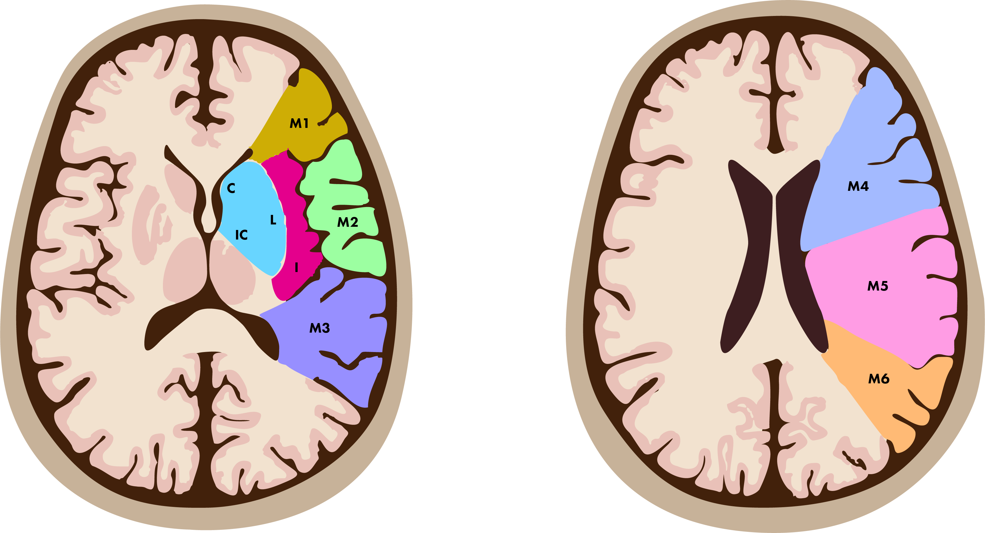
ASPECTS divides the MCA territory into 10 regions, with one point assigned to each region. Points are deducted for areas demonstrating evidence of ischemic change, such as hypodensity or loss of gray-white differentiation. The total score ranges from 0 to 10, where 10 indicates no ischemic changes and 0 represents extensive infarction involving the entire MCA territory [1].
The 10 regions evaluated in ASPECTS include the following:
- Subcortical regions: caudate, lentiform nucleus, and internal capsule.
- Cortical regions: insular ribbon, M1 through M6 regions (divisions of the MCA cortex from superior to inferior).
1.2 Clinical Relevance #
The ASPECTS score serves as an invaluable instrument in assessing the severity of stroke and consequently in forming treatment decisions. A score of ≤ 7 is linked to an elevated risk of adverse outcomes and hemorrhagic transformation subsequent to reperfusion therapies, such as intravenous thrombolysis or mechanical thrombectomy, as indicated by [1]. By offering a quantitative assessment of early ischemic alterations, ASPECTS enhances communication between healthcare professionals, assists in the identification of suitable candidates for further advanced imaging or therapeutic interventions, and plays a predictive role in determining the patient’s prognosis.
2. ASPECTS Region Labeling #
The primary objective of this phase of the project was to develop a comprehensive and broadly applicable segmentation pipeline for ASPECTS regions. The dataset available for this endeavor was comprised of DICOMDIR files from the KSSG, which included imaging data for approximately 2000 patients. However, it is important to note that a significant proportion of these scans did not include any ASPECTS region annotations. Specifically, out of the more than 50k CT scans in the repository, only about 1.67k scans were accompanied by ASPECTS region data, presented as a binary point cloud overlay.
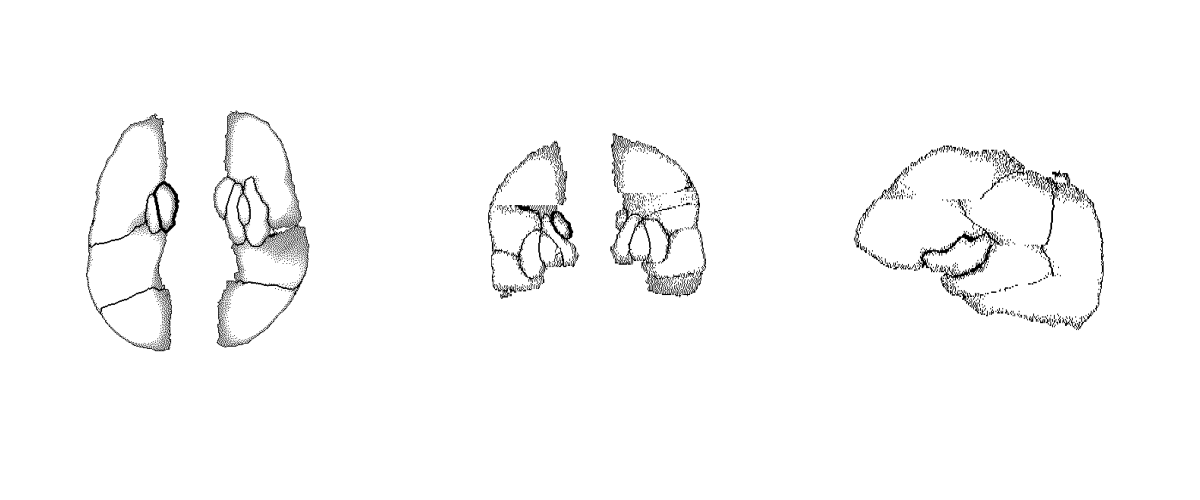
The baseline established by the existing point-cloud overlays was instrumental for deriving segmentation masks. However, initial methods employing morphological operations coupled with connected component analysis did not yield robust segmentation masks from the point cloud data. The primary difficulty stemmed from the fact that many current overlays exhibited substantial gaps or were entirely devoid of sections of the region outlines, as depicted below, where gaps and noisy borders are clearly visible. Although it was feasible to develop morphological operations tailored to function on certain overlays, a universally reliable and effective implementation of this technique proved unattainable.
2.1 Atlas-based Segmentation Mask Generation #
The definitive method adopted to ensure a consistent and universally reliable translation of overlay point clouds into filled segmentation masks specific to the ASPECTS region involved employing a sophisticated approach characterized by atlas-based registration using an aggressive variant of Symmetric Diffeomorphic Normalization (SyN) as described in the next section. In essence, the principal objective was to utilize a publicly available standardized brain template, referred to as an atlas, to systematically register all computed tomography (CT) scans containing point cloud overlays with said atlas. This registration process was followed by applying the resultant transformations to the overlays themselves in order to align them within a similar spatial domain, achieving maximum consistency across subjects. The registered and transformed overlays were subsequently integrated to construct a unified volumetric data set. All registered overlays were then used to generate a single volume, where each overlay was aggregated into a single mean overlay template.

Despite the aggregation of all overlays it was still not trivial to get a proper segmentation mask for the aggregated overlay using morphological operations. Therefore a 3D segmentation tool was used to manually annotate such a segmentation mask for the aggregated overlays, which resulted in a single, manually annotated, segmentation mask, that could be used as an atlas as well. Ultimately the process to get robust segmentation masks for each individual scan, containing ASPECTS region overlays (point clouds) was as following:
- Strip skull from raw CT scan - In order to make the registration more accurate, the skull was first stripped (leaving only brain tissue), using morphological operations.
- Register stripped CT with CT atlas - Using SyN and a publicly available brain CT atlas [2], the stripped CT scan was registered with the atlas.
- Transform overlay with outline of manually annotated segmentation mask atlas - Using SyN and the manually annotated segmentation mask outlines, the transformed overlay was registered once more, in order to get the best possible match between segmentation atlas and overlay.
- Inverse Transform of the Segmentation mask - The resulting transforms of the registration steps were then inversely applied to the segmentation atlas in order to map it to the raw CT spatial domain.
3. Symmetric Diffeomorphic Normalization (SyN) #
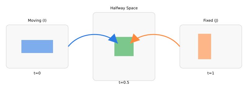
Diffeomorphic registration seeks a smooth, invertible deformation that aligns a moving image to a fixed image without tearing or folding anatomy. “Diffeomorphic” means the map is bijective and both it and its inverse are smooth; this preserves topology and enables meaningful inverse warps for region-of-interest (ROI) transfer or voxelwise analysis. SyN avoids bias toward either image by pushing both images into a halfway space. Intuitively, rather than warping only I to J, SyN finds two deformations that meet in the middle, so anatomical structures share the alignment burden. For NCCT brain scans—where intensity statistics are relatively consistent across subjects compared to multimodal settings—SyN paired with (localized) cross-correlation is well-suited: it is robust to global intensity offsets, emphasizes local structure, and keeps deformations smooth and invertible [3, 4].
3.1 Background: Diffeomorphic Flows and LDDMM #
Let be a flow of diffeomorphisms driven by a time-varying velocity in a reproducing-kernel Hilbert space :
The Reproducing Kernel Hilbert Space (RKHS) norm is induced by a (typically elliptic) operator with Green’s kernel , ensuring smooth vector fields and hence diffeomorphisms [5]. Classic Large deformation diffeomorphic metric mapping (LDDMM) minimizes the kinetic energy of the flow plus a data term:
The associated Euler–Lagrange equations yield momentum fields that are transported by the flow (the EPDiff equation), with terminal conditions determined by the image similarity gradient [5].
3.2 Symmetric Objective and Halfway Space #
SyN introduces symmetry by optimizing two flows that meet at a midpoint. One convenient formulation seeks maps such that and are similar in the halfway space, with a shared regularization:
with . At the optimum (under symmetry assumptions) one obtains a pair of inverse-consistent maps meeting at . Practical SyN solves this via greedy updates that alternately (i) compute similarity gradients in the halfway space, (ii) smooth them by , and (iii) compose small diffeomorphic updates in both directions [3].
3.3 Similarity Term for NCCT: Localized (Normalized) Cross-Correlation #
For same-modality NCCT, cross-correlation (CC) or localized normalized CC (LNCC) are standard and effective \cite{Avants.2008, Avants.2011}. Denote Gaussian smoothing by . Define local means , , and local second moments , , . The LNCC at voxel is:
and the image dissimilarity is . The gradient can be derived by quotient rule and chain rule through the local statistics; SyN’s implementation uses closed-form voxelwise expressions followed by convolutional smoothing to yield stable updates [3, 4].
3.4 Variational Derivatives and Updates (Sketch) #
Let , be the halfway-space images. Differentiating w.r.t.\ uses , yielding a force term in halfway space that is then pulled back to the domain of via the inverse deformation and Jacobian:
The velocity update applies the inverse of the regularizer (i.e., smoothing with ):
followed by composition of small diffeomorphic steps to keep invertibility: , . Here, denotes integration of the stationary substep (often via scaling-and-squaring). Writing (the momentum), EPDiff transport relates across time, which SyN approximates through its symmetric greedy scheme [3, 4].
3.5 Jacobian and Topology Control #
Diffeomorphism necessitates for all . In practice, SyN’s smoothing (via ) and step-size control stabilize updates. Post-hoc quality metrics include:
- Jacobian bounds - Monitor and to detect local folding.
- Inverse consistency - .
- Overlap/label metrics - Dice/Jaccard on neuroanatomical labels when available [6].
3.6 Why SyN for CT? #
SyN’s symmetry reduces template-selection bias; LNCC handles local contrast variability in NCCT; and the diffeomorphic constraint preserves anatomical topology while supporting inverse mapping for label transfer and voxelwise analyses [3, 4, 6].
4. ASPECTS Regions Segmentation using Deep Learning #
Annotating ASPECTS regions on raw NCCT brain scans can, in principle, be addressed through SyN registration against a curated ASPECTS atlas, as described earlier. However, this atlas-based strategy comes with significant drawbacks. Even in its optimized, aggressive form, a single SyN registration requires more than three minutes on high-end hardware (e.g., a 24-core CPU). In addition, a second registration step—aligning the transformed point-cloud overlay with the atlas outline—was only possible for NCCT scans that already included such overlays, which was rarely the case. While not strictly essential, this second pass appeared to improve segmentation accuracy, but at the cost of additional computation.
These limitations conflict directly with the clinical context in which ASPECTS is applied. In hyperacute stroke assessment, time is critical, and a segmentation pipeline that requires several minutes per scan is impractical. This is precisely where deep learning becomes valuable: it offers a way to achieve accurate ASPECTS region segmentation within seconds, enabling real-time decision support in acute care.
The SyN registration approach was used to curate a dataset, consisting of the following:
- raw_volumes / raw_segmentation - Containing the raw volumes (scans) as well as the corresponding curated segmentation masks, mapped back to the spatial domain of the raw volumes.
- stripped_volumes - Containing the raw volumes, with non-brain tissue masked out.
- registered_volumes / registered_segmentation - Containing the volumes, mapped to the spatial domain of the CT atlas and their corresponding curated segmentation masks.
3D U-Net Architecture #
In the previous project phase (Specialization Module 1), a library of 3D convolutional neural network (3D CNN) based custom pytorch modules were implemented and reused in this phase. Specifically:
- SqueezeExcite3D - A 3D adaptation of the Squeeze-and-Excitation (SE) block, introduced by [7], which helps the network foxus on the most important features in each channel.
- ResBlock3D - A 3D adaptation of residual blocks, which allow for deeper networks, using residual skip-connections [8].
- CNNEncoder3D - An encoder, using 3D convolutional layers (ResBlock3D layers) to produce latent representations of the input volumes.
- UNetEncoder3D - Extension of the CNNEncoder3D that exposes intermediate layers of the encoder as outputs.
- CNNDecoder3D - Uses 3D convolutional layers (ResBlock3D layers) to construct a volume from a latent representation. Can optionally use skip-connections from the encoder.
- UNet3D - A wrapper, implementing a UNet3D model, internally using UNetEncoder3D and CNNDecoder3D.

4.1 Loss and Metrics #
4.1.1 Dice CE Loss #
For training the UNet3D model, a composite loss function, \texttt{DiceCELoss}, from the MONAI library was employed. This loss function combines the Dice loss with the Cross-Entropy (CE) loss, leveraging the complementary strengths of both [9, 10].
Dice Loss - Intuition: Dice loss is derived from the Dice Similarity Coefficient (DSC), a set-overlap measure widely used in medical image analysis. Its key advantage is that it directly optimizes the volumetric overlap between the predicted segmentation and the ground truth . Intuitively, it answers:
“Of all voxels predicted for a given class, how many truly belong to that class — and vice versa?”
It is particularly robust to class imbalance: even if a class occupies only a small fraction of the image, its contribution to the loss is not overwhelmed by large background regions.
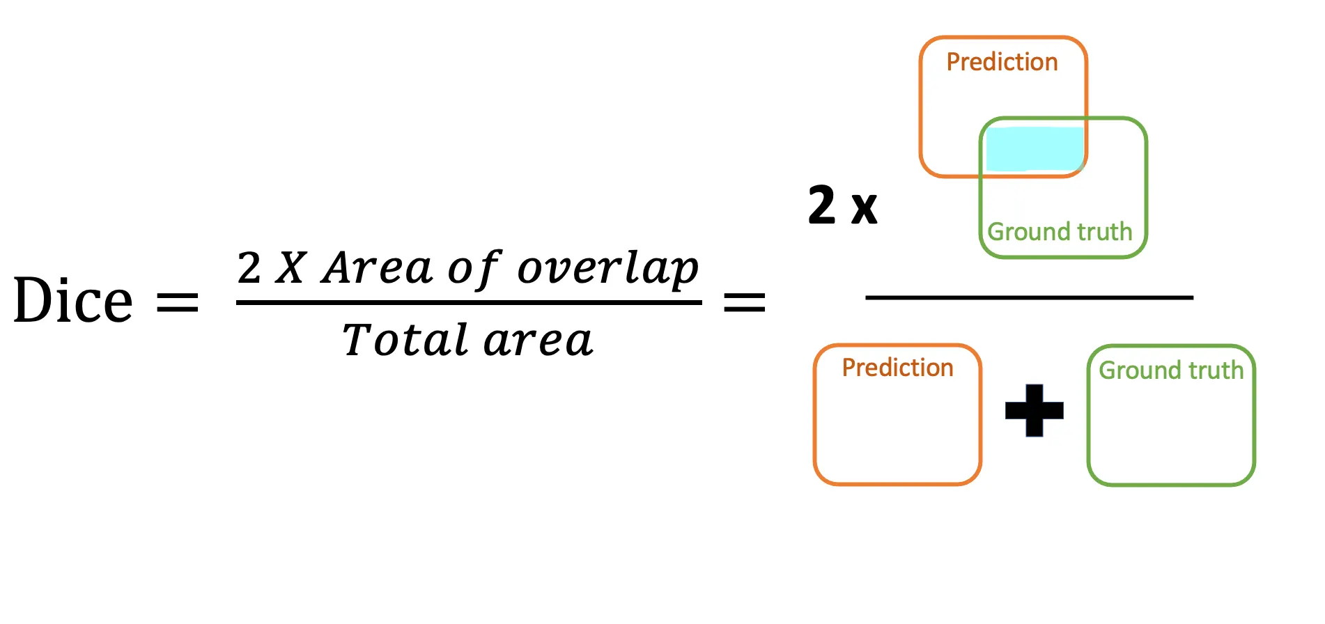
Mathematically, the Dice loss for classes is:
where is the number of voxels, and are the ground truth and predicted probabilities for voxel and class , and is a small constant for numerical stability.
The total loss used is:
with and , computed on one-hot encoded labels, including the background class, and with a sigmoid activation applied to the model output. The Dice term drives the model to maximize region overlap, while the CE term enforces voxel-wise correctness.
4.1.2 Generalized Dice Score #
The standard Dice score can still be biased toward large structures, as their overlaps dominate the global average. The \emph{Generalized Dice Score} (GDS) addresses this by weighting each class inversely to the square of its volume in the ground truth [9]. This ensures that small but clinically important regions have equal influence during evaluation. Formally:
with weights:
5. Training and Results #
The final model was trained on the DGX-2 cluster on 8 Nvidia V100 GPUs, with early stopping (based on val/dice_mean) and patience of 10. The dataset consisted of a total of 4971 input/label pairs, in equal parts containing raw volumes, stripped volumes and registered volumes. The model was trained on these different stages (raw, stripped and registered), to enforce more diverse input (beyond simple augmentation) and thus acquire a stronger, more generalized final model.
| Hyperparameter | Value |
|---|---|
| Learning Rate | 1e-3 |
| Test Size | 0.1 |
| Batch Size | 2 |
| Volume Size | 256 |
| Number of Workers | 8 |
| Number of Epochs | 300 |
| Base Channels | 8 |
| Dropout | 0.2 |
| Strategy | fsdp |
| Use SE | True |
| Skip Validation | True |
| Use Augments | True |
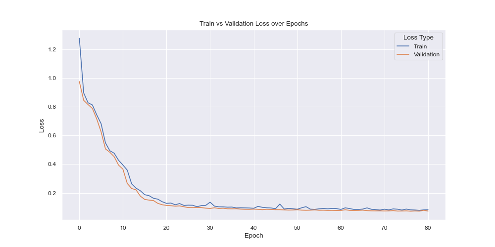
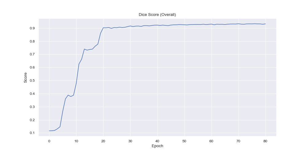
As depicted above, both training and evaluation losses were consistently going down and no sign of overfitting (based on loss) was visually present.
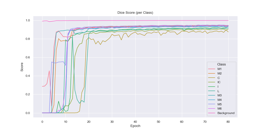
From the per-class dice score visualization it is evident that the model had the easiest time to label the background correctly, which is an expected behaviour since it is arguably the easiest (everything that is not brain tissue) and also it is the largest region by a big margin. Over time however the smaller region predictions became more and more accurate with the smallest of them (C, IC, I and L) expectedly having the latest rises in the dice score, due to their small and complicated nature.
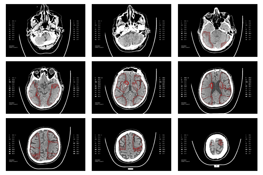
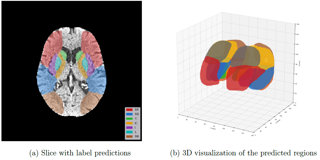
Below, the predicted ASPECTS regions of a validation sample on a single slice and the entire predicted volume is visualized.

The final model performance was as follows:
| Statistic | Value |
|---|---|
| epoch | 68 |
| train/loss | 0.0862 |
| val/loss | 0.0737 |
| val/dice_mean | 0.9324 |
| val/dice_0 | 0.9454 |
| val/dice_1 | 0.9423 |
| val/dice_2 | 0.8746 |
| val/dice_3 | 0.9055 |
| val/dice_4 | 0.9183 |
| val/dice_5 | 0.9182 |
| val/dice_6 | 0.9348 |
| val/dice_7 | 0.9335 |
| val/dice_8 | 0.9454 |
| val/dice_9 | 0.9398 |
| val/dice_10 | 0.9983 |
6. Conclusion #
This second phase of the DeepStroke project successfully demonstrated that sparse, heterogeneous clinical annotations—such as legacy ASPECTS point-cloud overlays—can be transformed into robust, volumetric ground truth suitable for training high-performance 3D segmentation models. By integrating a reproducible DICOMDIR-to-NIfTI conversion pipeline, atlas-based registration using Symmetric Diffeomorphic Normalization (SyN), and label back-projection to native space, the methodology ensured spatial consistency across a diverse dataset of around 1700 annotated NCCT series.
The curated dataset enabled the training of a configurable 3D U-Net, optimized using a DiceCE loss to balance overlap maximization and voxel-wise accuracy, and evaluated with a class-balanced Generalized Dice Score. Leveraging FSDP-based multi-GPU training on the DGX-2 cluster allowed for efficient scaling and large-volume processing, achieving a mean Dice score of 0.9324 across all ASPECTS regions. Performance was strongest in larger anatomical areas, with steady improvement in smaller, anatomically complex regions throughout training.
Beyond its quantitative results, the project contributes a modular, end-to-end framework for standardized NCCT preprocessing, label harmonization, and volumetric segmentation. By bridging the gap between noisy clinical annotations and research-grade training labels, this work advances the feasibility of scalable, automated ASPECTS scoring and holds promise for integration into acute stroke decision support systems.
7. Next Steps for the DeepStroke Project #
Building upon the results and infrastructure developed in this phase, the following final phase is proposed to advance the DeepStroke project toward clinically deployable, extended functionality:
-
Segmentation Model Analysis
The final model will be analyzed in detail, with a focus on error cases and confidence estimation. Additionally, performance will be benchmarked against other state-of-the-art architectures, such as SwinUNETR. -
ASPECTS Score Prediction from Automated Segmentations
Leveraging the automatically segmented ASPECTS regions produced by the UNet-3D model, a range of machine learning (ML) algorithms will be trained and hyperparameter-optimized to directly predict the ASPECTS score. Model performance will be evaluated against ground-truth clinical scores, establishing a fully automated end-to-end pipeline from NCCT to ASPECTS score. -
Extension of the ASPECTS Scoring Framework
The traditional HU-based ASPECTS evaluation will be extended with additional structural and statistical descriptors from the segmented regions, including volumetric shape metrics, intensity distributions, and texture features. The extended scoring system will be quantitatively compared to the standard approach to assess its potential for improved prognostic accuracy. -
Publication I
The methodologies and findings from steps (2) and (3) will be prepared for dissemination in a peer-reviewed journal or presented at a scientific conference. -
Ischemic Stroke Detection and Localization
A dedicated neural network will be developed for the detection and spatial localization of ischemic stroke lesions (thrombotic or embolic occlusions). Training and validation will be conducted on labeled CT datasets, including both standard NCCT and CT angiography. This work will extend the system beyond ASPECTS scoring toward comprehensive stroke diagnosis support. -
Documentation and Presentation
Comprehensive project documentation will be produced, along with a well-structured GitLab repository containing all developed and adapted code. The thesis will culminate in an expert-level presentation of results, methodologies, and implications for clinical translation.
References #
[1] Anne G. Osborn. Osborn’s Brain. 3rd edition. Philadelphia: Elsevier, 2024. isbn: 9780443109379. url: https://permalink.obvsg.at/AC17026293. [2] GitHub. muschellij2/high_res_ct_template: High Resolution CT Template Paper and Images. 8/9/2025. url: https://github.com/muschellij2/high_res_ct_template. [3] B. B. Avants et al. “Symmetric diffeomorphic image registration with cross-correlation: evaluating automated labeling of elderly and neurodegenerative brain”. In: Medical image analysis 12.1 (2008), pp. 26–41. doi: 10.1016/j.media.2007.06.004. url: https://www.sciencedirect.com/science/article/pii/S1361841507000606. [4] Brian B. Avants et al. “A reproducible evaluation of ANTs similarity metric performance in brain image registration”. In: NeuroImage 54.3 (2011), pp. 2033–2044. doi: 10.1016/j.neuroimage.2010.09.025.s [5] M. Faisal Beg et al. “Computing Large Deformation Metric Mappings via Geodesic Flows of Diffeomorphisms”. In: International Journal of Computer Vision 61.2 (2005), pp. 139–157. issn: 0920-5691. doi: 10.1023/B:VISI.0000043755.93987.aa. url: https://link.springer.com/article/10.1023/B:VISI.0000043755.93987.aa. [6] Arno Klein et al. “Evaluation of 14 nonlinear deformation algorithms applied to human brain MRI registration”. In: NeuroImage 46.3 (2009), pp. 786–802. doi: 10.1016/j. neuroimage.2008.12.037. url: https://pmc.ncbi.nlm.nih.gov/articles/PMC2747506/ [7] Jie Hu et al. Squeeze-and-Excitation Networks. url: http://arxiv.org/pdf/1709.01507. [8] Kaiming He et al. Deep Residual Learning for Image Recognition. url: http://arxiv.org/pdf/1512.03385. [9] Carole H. Sudre et al. Generalised Dice Overlap as a Deep Learning Loss Function for Highly Unbalanced Segmentations. 2017. doi: 10.1007/978-3-319-67558-9_28. url: http://arxiv.org/pdf/1707.03237. [10] Project MONAI — MONAI 1.4.0 Documentation. 16.10.2024. url: https://docs.monai.io/en/stable/.